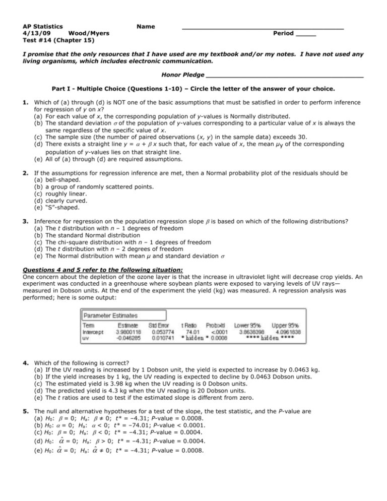
AP Statistics
4/13/09
Wood/Myers
Test #14 (Chapter 15)
Name
________________________________________
Period _____
I promise that the only resources that I have used are my textbook and/or my notes. I have not used any
living organisms, which includes electronic communication.
Honor Pledge _______________________________________
Part I - Multiple Choice (Questions 1-10) – Circle the letter of the answer of your choice.
1. Which of (a) through (d) is NOT one of the basic assumptions that must be satisfied in order to perform inference
for regression of y on x?
(a) For each value of x, the corresponding population of y-values is Normally distributed.
(b) The standard deviation  of the population of y-values corresponding to a particular value of x is always the
same regardless of the specific value of x.
(c) The sample size (the number of paired observations (x, y) in the sample data) exceeds 30.
(d) There exists a straight line y =  +  x such that, for each value of x, the mean µy of the corresponding
population of y-values lies on that straight line.
(e) All of (a) through (d) are required assumptions.
2. If the assumptions for regression inference are met, then a Normal probability plot of the residuals should be
(a) bell-shaped.
(b) a group of randomly scattered points.
(c) roughly linear.
(d) clearly curved.
(e) “S”-shaped.
3. Inference for regression on the population regression slope  is based on which of the following distributions?
(a) The t distribution with n – 1 degrees of freedom
(b) The standard Normal distribution
(c) The chi-square distribution with n – 1 degrees of freedom
(d) The t distribution with n – 2 degrees of freedom
(e) The Normal distribution with mean µ and standard deviation 
Questions 4 and 5 refer to the following situation:
One concern about the depletion of the ozone layer is that the increase in ultraviolet light will decrease crop yields. An
experiment was conducted in a greenhouse where soybean plants were exposed to varying levels of UV rays—
measured in Dobson units. At the end of the experiment the yield (kg) was measured. A regression analysis was
performed; here is some output:
4. Which of the following is correct?
(a) If the UV reading is increased by 1 Dobson unit, the yield is expected to increase by 0.0463 kg.
(b) If the yield increases by 1 kg, the UV reading is expected to decline by 0.0463 Dobson units.
(c) The estimated yield is 3.98 kg when the UV reading is 0 Dobson units.
(d) The predicted yield is 4.3 kg when the UV reading is 20 Dobson units.
(e) The t ratios are used to test if the estimated slope is different from zero.
5. The null and alternative hypotheses for a test of the slope, the test statistic, and the P-value are
(a) H0:  = 0; Ha:  ≠ 0; t* = –4.31; P-value = 0.0008.
(b) H0:  = 0; Ha:  < 0; t* = –74.01; P-value < 0.0001.
(c) H0:  = 0; Ha:  < 0; t* = –4.31; P-value = 0.0004.
(d) H0:
(e) H0:
̂ = 0; Ha:  > 0; t* = –4.31; P-value = 0.0004.
̂ = 0; Ha: ̂ ≠ 0; t* = –4.31; P-value = 0.0008.
6. If a test of hypotheses rejects H0:  = 0 in favor of the alternative hypothesis Ha:  > 0, where  is the population
regression slope, then the least-squares regression line
(a) is useful for predicting y, given x (within the limits of x-values covered by the data).
(b) slopes downward and to the right when plotted on the scatterplot of paired observations (x, y).
(c) can be extrapolated beyond the limits of the x-values covered by the data to predict y at any possible x.
(d) is not useful for predicting y, given x.
(e) has an intercept that is greater than zero.
The following information is used in Questions 7 and 8.
A random sample of 80 companies from the Forbes 500 list was selected and the relationship between sales (in
hundreds of thousands of dollars) and profits (in hundreds of thousands of dollars) was investigated by regression. A
least-squares regression line was fitted to the data using statistical software, with sales as the explanatory variable
and profits as the response variable. Here is the output from the software:
Dependent variable is Profits
R squares = 66.2%
s = 466.2 with 80 – 2 = 78 degrees of freedom
Variable
Constant
Sales
Coefficient
–176.644
0.092498
s.e. of Coefficient P-value
61.16
0.0050
0.0075
≤0.0001
7.
Using the above data, approximately what is a 90% confidence interval for the slope of the least-squares
regression line?
(a) 0.0925 ± 0.0075
(b) 0.0925 ± 0.012
(c) –0.0925 ± 0.0075
(d) –0.0925 ± 0.012
(e) None of the above.
8.
Using the above data, is there strong evidence (and if so, why) of a straight-line relationship between sales and
profits?
(a) Yes, because the slope of the least-squares line is positive.
(b) Yes, because the P-value for testing if the slope is 0 is quite small.
(c) No, because the value of the square of the correlation is relatively small.
(d) It is impossible to say because we are not given the actual value of the correlation.
(e) None of the above.
The following information is used in Questions 9 and 10.
A marine biologist wants to test the effect of water temperature on the average dive duration for sea otters. Several
otters are available for an experiment. The biologist collects the following data:
Otter
J2
J1
B7
B9
M3
D4
B8
Water
Dive
temp.(C) duration (sec)
x
y
4
63
8
75
8
84
12
91
12
101
16
110
20
115
We want to determine if water temperature is useful in
predicting dive duration. Here is output from Minitab for
these data:
Predictor
Constant
H2Otemp
s = 5.557
Coef
52.789
3.3684
Stdev
5.257
0.4216
R-sq = 92.7%
t-ratio
10.04
***
R-sq(adj) = 91.3%
9. The t statistic for testing H0 has been left out. From the output, the t-statistic has the value
(a) 7.99.
(b) 10.04.
(c) 0.124.
(d) 0.927.
(e) 15.67.
10. The P-value is
(a) less than 0.001.
(b) between 0.001 and 0.01.
(c) between 0.01 and 0.05.
(d) between 0.05 and 0.10.
(e) greater than 0.10.
p
0.000
***
Part II – Free Response (Question 11-12) – Show your work and explain your results clearly.
11. A teacher asked her 8 introductory statistics students to record the total amount of time
they spent studying for a particular test. The amounts of study time x (in hours) and
the resulting test grades y are given below.
x
2
1
1.5
0.5
1
3
0
2
y
92
81
84
68
85
96
48
74
(a) Make a scatterplot of the data.
(b) Use your calculator to obtain the equation of the least-squares regression line and
the correlation.
(c)
Explain in words what the slope b of the least-squares line says about hours studied
and grade awarded.
(d) What is the estimate of  from the data? What is your estimate of the intercept  of the true regression
line?
(e) Use your calculator to calculate the residuals. Report the sum of the residuals and the sum of the squares
of the residuals. Then use these results to estimate the standard deviation  in the regression model.
Interpret this value in context.
(f)
Calculate and interpret SEb.
(g) Do we have evidence that the number of hours studied helps predict grade awarded on this statistics test?
12. A mathematics professor wishes to analyze the relationship between the number of papers (in hundreds) graded
by his department’s student homework graders and the total amount of money paid to the graders. He collects
data for 12 randomly chosen graders and uses MINITAB to do regression analysis. Below is a portion of the
Minitab output. (Here, COST = amount paid (dollars), PAPERS = number of papers in hundreds, and the intervals
listed at the bottom are computed for 1600 papers.)
The regression equation is
COST = 35.8 + 12.1 PAPERS
Predictor
Constant
PAPERS
s = 6.526
Coef
35.80
12.0835
Stdev
17.06
0.9738
t-ratio
2.10
12.41
R-sq = 93.9%
P
0.062
0.000
R-sq (adj) = 93.3%
(a) What is the least-squares regression equation?
(c) What is the standard deviation s in the regression model? Interpret this value in context.
(d) Interpret the slope of the least-squares regression line in the context of this problem.
(e) The model for regression inference has three parameters: , , and . Estimate these parameters from the
data.
(f) Calculate and interpret a 95% confidence interval on the slope of the least-squares regression line