AP Statistics: Hypothesis Testing Notes
advertisement
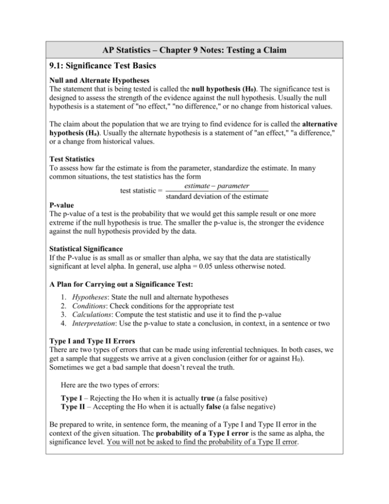
AP Statistics – Chapter 9 Notes: Testing a Claim 9.1: Significance Test Basics Null and Alternate Hypotheses The statement that is being tested is called the null hypothesis (H0). The significance test is designed to assess the strength of the evidence against the null hypothesis. Usually the null hypothesis is a statement of "no effect," "no difference," or no change from historical values. The claim about the population that we are trying to find evidence for is called the alternative hypothesis (Ha). Usually the alternate hypothesis is a statement of "an effect," "a difference," or a change from historical values. Test Statistics To assess how far the estimate is from the parameter, standardize the estimate. In many common situations, the test statistics has the form estimate parameter test statistic = standard deviation of the estimate P-value The p-value of a test is the probability that we would get this sample result or one more extreme if the null hypothesis is true. The smaller the p-value is, the stronger the evidence against the null hypothesis provided by the data. Statistical Significance If the P-value is as small as or smaller than alpha, we say that the data are statistically significant at level alpha. In general, use alpha = 0.05 unless otherwise noted. A Plan for Carrying out a Significance Test: 1. 2. 3. 4. Hypotheses: State the null and alternate hypotheses Conditions: Check conditions for the appropriate test Calculations: Compute the test statistic and use it to find the p-value Interpretation: Use the p-value to state a conclusion, in context, in a sentence or two Type I and Type II Errors There are two types of errors that can be made using inferential techniques. In both cases, we get a sample that suggests we arrive at a given conclusion (either for or against H0). Sometimes we get a bad sample that doesn’t reveal the truth. Here are the two types of errors: Type I – Rejecting the Ho when it is actually true (a false positive) Type II – Accepting the Ho when it is actually false (a false negative) Be prepared to write, in sentence form, the meaning of a Type I and Type II error in the context of the given situation. The probability of a Type I error is the same as alpha, the significance level. You will not be asked to find the probability of a Type II error. 9.2: Tests about a Population Proportion Z-test for a Population Proportion (one-proportion z-test) 1. Hypotheses: H0: 𝑝 = 𝑝0 ; Ha: 𝑝 < 𝑝0 or 𝑝 > 𝑝0 or 𝑝 ≠ 𝑝0 2. Conditions: o Random – does the data come from a random sample? o Independent – is the sample size less than 10% of the population size? o Normal – Are np0 and n(1 p0 ) both at least 10? 3. Test-Statistic: 𝑧 = 𝑝̂−𝑝0 𝑝 (1−𝑝0 ) √ 0 where 𝑝̂ is the sample proportion 𝑛 P-value: The P-value is based on a normal z-distribution. This value can be estimated using Table A or found accurately using the 1-Prop Z-test function on your calculator 4. Conclusion: If P < , then Reject the H0, otherwise Fail to Reject H0. 9.3: Tests about a Population Mean T-test for a Population Mean 1. Hypotheses: H0: = 0; Ha: < 0 or > 0 or 0 2. Conditions: o Random – does the data come from a random sample? o Independent – is the sample size less than 10% of the population size? o Normal – Is it given or is there a large sample size ( n 30 )? 𝑥̅ −𝜇 3. Test-Statistic: 𝑡 = 𝑠 0where s is the sample standard deviation ⁄ 𝑛 √ P-value: The P-value is based on a t-distribution with n 1 degrees of freedom. This value can be estimated using Table C or found accurately using the T-test function on your calculator 4. Conclusion: If P < , then Reject the H0, otherwise Fail to Reject H0. Paired Differences T-test To compare the responses to the two treatments in a paired data design, apply the one-sample t procedures to the observed differences. For example, suppose that pre and post test scores for 10 individuals in a summer reading program are: Subject Pre-test Post-test Difference 1 25 28 3 2 31 30 -1 3 28 34 6 4 27 35 8 5 30 32 2 6 31 31 0 7 22 26 4 8 18 16 -2 9 24 28 4 We would use the data in the differences row and perform one-sample t analysis on it. 10 30 36 6
