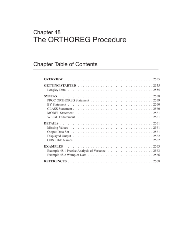
Chapter 48
The ORTHOREG Procedure
Chapter Table of Contents
OVERVIEW . . . . . . . . . . . . . . . . . . . . . . . . . . . . . . . . . . . 2555
GETTING STARTED . . . . . . . . . . . . . . . . . . . . . . . . . . . . . . 2555
Longley Data . . . . . . . . . . . . . . . . . . . . . . . . . . . . . . . . . . 2555
SYNTAX . . . . . . . . . . . .
PROC ORTHOREG Statement
BY Statement . . . . . . . . .
CLASS Statement . . . . . . .
MODEL Statement . . . . . .
WEIGHT Statement . . . . .
.
.
.
.
.
.
.
.
.
.
.
.
.
.
.
.
.
.
.
.
.
.
.
.
.
.
.
.
.
.
.
.
.
.
.
.
.
.
.
.
.
.
.
.
.
.
.
.
.
.
.
.
.
.
.
.
.
.
.
.
.
.
.
.
.
.
.
.
.
.
.
.
.
.
.
.
.
.
.
.
.
.
.
.
.
.
.
.
.
.
.
.
.
.
.
.
.
.
.
.
.
.
.
.
.
.
.
.
.
.
.
.
.
.
.
.
.
.
.
.
.
.
.
.
.
.
.
.
.
.
.
.
.
.
.
.
.
.
.
.
.
.
.
.
. 2558
. 2559
. 2560
. 2560
. 2561
. 2561
DETAILS . . . . . .
Missing Values . .
Output Data Set . .
Displayed Output .
ODS Table Names
.
.
.
.
.
.
.
.
.
.
.
.
.
.
.
.
.
.
.
.
.
.
.
.
.
.
.
.
.
.
.
.
.
.
.
.
.
.
.
.
.
.
.
.
.
.
.
.
.
.
.
.
.
.
.
.
.
.
.
.
.
.
.
.
.
.
.
.
.
.
.
.
.
.
.
.
.
.
.
.
.
.
.
.
.
.
.
.
.
.
.
.
.
.
.
.
.
.
.
.
.
.
.
.
.
.
.
.
.
.
.
.
.
.
.
.
.
.
.
.
. 2561
. 2561
. 2561
. 2562
. 2562
.
.
.
.
.
.
.
.
.
.
.
.
.
.
.
.
.
.
.
.
.
.
.
.
.
.
.
.
.
.
EXAMPLES . . . . . . . . . . . . . . . . . . . . . . . . . . . . . . . . . . . 2563
Example 48.1 Precise Analysis of Variance . . . . . . . . . . . . . . . . . . 2563
Example 48.2 Wampler Data . . . . . . . . . . . . . . . . . . . . . . . . . . 2566
REFERENCES . . . . . . . . . . . . . . . . . . . . . . . . . . . . . . . . . . 2568
2554 Chapter 48. The ORTHOREG Procedure
SAS OnlineDoc: Version 8
Chapter 48
The ORTHOREG Procedure
Overview
The ORTHOREG procedure fits general linear models by the method of least squares.
Other SAS/STAT software procedures, such as GLM or REG, fit the same types of
models, but PROC ORTHOREG can produce more accurate estimates than other
regression procedures when your data are ill conditioned. Instead of collecting
crossproducts, PROC ORTHOREG uses Gentleman-Givens transformations to update and compute the upper triangular matrix of the QR decomposition of the data
matrix, with special care for scaling (Gentleman 1972; 1973). This method has the
advantage over other orthogonalization methods (for example, Householder transformations) of not requiring the data matrix to be stored in memory.
R
The standard SAS regression procedures (REG and GLM) are very accurate for most
problems. However, if you have very ill-conditioned data, these procedures can produce estimates that yield an error sum of squares very close to the minimum but still
different from the exact least-squares estimates. Normally, this coincides with estimates that have very high standard errors. In other words, the numerical error is much
smaller than the statistical standard error.
Note that PROC ORTHOREG fits models by the method of linear least squares, minimizing the sum of the squared residuals for predicting the responses. It does not
perform the modeling method known as “orthogonal regression,” which minimizes
a different criterion (the distance between the X/Y points taken together and the regression line.)
Getting Started
Longley Data
The labor statistics data set of Longley (1967) is noted for being ill conditioned. Both
the ORTHOREG and GLM procedures are applied for comparison (only portions of
the PROC GLM results are shown). Note: The results from this example vary from
machine to machine, depending on floating-point configuration.
The following statements read the data into the SAS data set Longley.
2556 Chapter 48. The ORTHOREG Procedure
title ’PROC ORTHOREG used with Longley data’;
data Longley;
input Employment Prices GNP Jobless Military PopSize Year;
datalines;
60323 83.0 234289 2356 1590 107608 1947
61122 88.5 259426 2325 1456 108632 1948
60171 88.2 258054 3682 1616 109773 1949
61187 89.5 284599 3351 1650 110929 1950
63221 96.2 328975 2099 3099 112075 1951
63639 98.1 346999 1932 3594 113270 1952
64989 99.0 365385 1870 3547 115094 1953
63761 100.0 363112 3578 3350 116219 1954
66019 101.2 397469 2904 3048 117388 1955
67857 104.6 419180 2822 2857 118734 1956
68169 108.4 442769 2936 2798 120445 1957
66513 110.8 444546 4681 2637 121950 1958
68655 112.6 482704 3813 2552 123366 1959
69564 114.2 502601 3931 2514 125368 1960
69331 115.7 518173 4806 2572 127852 1961
70551 116.9 554894 4007 2827 130081 1962
;
run;
The data set contains one dependent variable, Employment (total derived employment) and six independent variables: Prices (GNP implicit price deflator with year
1954 = 100), GNP (gross national product), Jobless (unemployment), Military (size
of armed forces), PopSize (non-institutional population aged 14 and over), and Year
(year).
The following statements use the ORTHOREG procedure to model the Longley data
using a quadratic model in each independent variable, without interaction:
proc orthoreg data=Longley;
model Employment = Prices
GNP
Jobless
Military
PopSize
Year
run;
Figure 48.1 shows the resulting analysis.
SAS OnlineDoc: Version 8
Prices*Prices
GNP*GNP
Jobless*Jobless
Military*Military
PopSize*PopSize
Year*Year;
Longley Data
2557
PROC ORTHOREG used with Longley data
ORTHOREG Regression Procedure
Dependent Variable: Employment
Source
DF
Sum of
Squares
Model
Error
Corrected Total
12
3
15
184864508.5
144317.49568
185008826
Root MSE
R-Square
Parameter
Intercept
Prices
Prices**2
GNP
GNP**2
Jobless
Jobless**2
Military
Military**2
PopSize
PopSize**2
Year
Year**2
Mean Square
F Value
Pr > F
15405375.709
48105.831895
320.24
0.0003
219.33041717
0.9992199426
DF
Parameter Estimate
Standard
Error
t Value
Pr > |t|
1
1
1
1
1
1
1
1
1
1
1
1
1
186931078.640216
1324.50679362506
-6.61923922845539
-0.12768642156232
3.1369569286212E-8
-4.35507653558708
0.00022132944101
4.91162014560828
-0.00113707146734
-0.0303997234299
-1.212511414607E-6
-194907.139041839
50.8067603538501
154201839.66
916.17455832
4.7891445654
0.0738897784
8.7167753E-8
1.3851792402
0.0001763541
1.826715856
0.0003539971
5.9272538242
0.0000237262
157739.28757
40.279878943
1.21
1.45
-1.38
-1.73
0.36
-3.14
1.26
2.69
-3.21
-0.01
-0.05
-1.24
1.26
0.3122
0.2440
0.2609
0.1824
0.7428
0.0515
0.2983
0.0745
0.0489
0.9962
0.9625
0.3045
0.2963
Figure 48.1.
PROC ORTHOREG Results
The estimates in Figure 48.1 compare very well with the best estimates available;
for additional information, refer to Longley (1967) and Beaton, Rubin, and Barone
(1976).
The following statements request the same analysis from the GLM procedure:
ods select OverallANOVA
FitStatistics
ParameterEstimates;
proc glm data=Longley;
model Employment = Prices
GNP
Jobless
Military
PopSize
Year
run;
Prices*Prices
GNP*GNP
Jobless*Jobless
Military*Military
PopSize*PopSize
Year*Year;
Figure 48.2 contains the over-all ANOVA table and the parameter estimates produced
by PROC GLM. Notice that the ORTHOREG fit achieves a somewhat smaller root
mean square error (RMSE) and also that the GLM procedure detects spurious singularities.
SAS OnlineDoc: Version 8
2558 Chapter 48. The ORTHOREG Procedure
PROC ORTHOREG used with Longley data
The GLM Procedure
Dependent Variable: Employment
Source
DF
Sum of
Squares
Mean Square
F Value
Pr > F
Model
11
184791061.6
16799187.4
308.58
<.0001
Error
4
217764.4
54441.1
15
185008826.0
Corrected Total
R-Square
Coeff Var
Root MSE
Employment Mean
0.998823
0.357221
233.3262
65317.00
Parameter
Intercept
Prices
Prices*Prices
GNP
GNP*GNP
Jobless
Jobless*Jobless
Military
Military*Military
PopSize
PopSize*PopSize
Year
Year*Year
Standard
Error
t Value
Pr > |t|
1327335.652
688.979
3.507
0.078
0.000
1.459
0.000
1.942
0.000
5.156
0.000
.
0.419
-2.71
0.76
-0.66
-1.76
0.24
-3.15
1.14
2.57
-3.15
-0.82
0.81
.
2.48
0.0535
0.4894
0.5434
0.1526
0.8218
0.0344
0.3183
0.0619
0.0346
0.4565
0.4655
.
0.0683
Estimate
-3598851.899 B
523.802
-2.326
-0.138
0.000
-4.599
0.000
4.994
-0.001
-4.246
0.000 B
0.000 B
1.038
NOTE: The X’X matrix has been found to be singular, and a generalized inverse
was used to solve the normal equations. Terms whose estimates are
followed by the letter ’B’ are not uniquely estimable.
Figure 48.2.
Partial PROC GLM Results
Syntax
The following statements are available in PROC ORTHOREG.
PROC ORTHOREG < options > ;
MODEL dependent=independents < / option > ;
BY variables ;
CLASS variables ;
WEIGHT variable ;
The BY, CLASS, MODEL, and WEIGHT statements are described after the PROC
ORTHOREG statement.
SAS OnlineDoc: Version 8
PROC ORTHOREG Statement
2559
PROC ORTHOREG Statement
PROC ORTHOREG < options > ;
The PROC ORTHOREG statement has the following options:
DATA=SAS-data-set
specifies the input SAS data set to use. By default, the procedure uses the most
recently created SAS data set. The data set specified cannot be a TYPE=CORR,
TYPE=COV, or TYPE=SSCP data set.
NOPRINT
suppresses the normal display of results. Note that this option temporarily disables
the Output Delivery System (ODS); see Chapter 15, “Using the Output Delivery
System,” for more information.
ORDER=DATA | FORMATTED | FREQ | INTERNAL
specifies the order in which you want the levels of the classification variables (specified in the CLASS statement) to be sorted. This ordering determines which parameters in the model correspond to each level in the data. Note that the ORDER=
option applies to the levels for all classification variables. The exception is ORDER=FORMATTED (the default) for numeric variables for which you have supplied
no explicit format (that is, for which there is no corresponding FORMAT statement in
the current PROC ORTHOREG run or in the DATA step that created the data set). In
this case, the levels are ordered by their internal (numeric) value. Note that this represents a change from previous releases for how class levels are ordered. In releases
previous to Version 8, numeric class levels with no explicit format were ordered by
their BEST12. formatted values, and in order to revert to the previous ordering you
can specify this format explicitly for the affected classification variables. The change
was implemented because the former default behavior for ORDER=FORMATTED
often resulted in levels not being ordered numerically and usually required the user
to intervene with an explicit format or ORDER=INTERNAL to get the more natural
ordering.
The ORDER= option can take the following values.
Value of ORDER=
DATA
Levels Sorted By
order of appearance in the input data set
FORMATTED
external formatted value, except for numeric
variables with no explicit format, which are
sorted by their unformatted (internal) value
FREQ
descending frequency count; levels with the
most observations come first in the order
INTERNAL
unformatted value
If you omit the ORDER= option, PROC ORTHOREG orders by the external formatted value.
SAS OnlineDoc: Version 8
2560 Chapter 48. The ORTHOREG Procedure
OUTEST=SAS-data-set
produces an output data set containing the parameter estimates, the BY variables, and
the special variables – TYPE– (value PARMS), – NAME– (blank), – RMSE– (root
mean squared error), and Intercept.
SINGULAR=s
specifies a singularity criterion (s By default, SINGULAR=10E,12.
0)
for the inversion of the triangular matrix
R.
BY Statement
BY variables ;
You can specify a BY statement with PROC ORTHOREG to obtain separate analyses on observations in groups defined by the BY variables. When a BY statement
appears, the procedure expects the input data set to be sorted in order of the BY
variables.
If your input data set is not sorted in ascending order, use one of the following alternatives:
Sort the data using the SORT procedure with a similar BY statement.
Specify the BY statement option NOTSORTED or DESCENDING in the BY
statement for the ORTHOREG procedure. The NOTSORTED option does not
mean that the data are unsorted but rather that the data are arranged in groups
(according to values of the BY variables) and that these groups are not necessarily in alphabetical or increasing numeric order.
Create an index on the BY variables using the DATASETS procedure (in base
SAS software).
For more information on the BY statement, refer to the discussion in SAS Language
Reference: Concepts. For more information on the DATASETS procedure, refer to
the discussion in the SAS Procedures Guide.
CLASS Statement
CLASS variables ;
The CLASS statement names the classification variables to be used in the model.
Typical class variables are Treatment, Sex, Race, Group, and Replication. If you
use the CLASS statement, it must appear before the MODEL statement.
Class levels are determined from up to the first 16 characters of the formatted values
of the CLASS variables. Thus, you can use formats to group values into levels.
Refer to the discussion of the FORMAT procedure in the SAS Procedures Guide
and the discussions for the FORMAT statement and SAS formats in SAS Language
Reference: Dictionary.
SAS OnlineDoc: Version 8
Output Data Set
2561
MODEL Statement
MODEL dependent=independents < / option > ;
The MODEL statement names the dependent variable and the independent effects.
Only one MODEL statement is allowed. The specification of effects and the parameterization of the linear model is the same as in the GLM procedure; see Chapter 30, “The GLM Procedure,” for further details.
The following option can be used in the MODEL statement:
NOINT
omits the intercept term from the model.
WEIGHT Statement
WEIGHT variable ;
A WEIGHT statement names a variable in the input data set whose values are relative
weights for a weighted least-squares regression. If the weight value is proportional to
the reciprocal of the variance for each observation, the weighted estimates are the best
linear unbiased estimates (BLUE). For a more complete description of the WEIGHT
statement, see Chapter 30.
Details
Missing Values
If there is a missing value for any model variable in an observation, the entire observation is dropped from the analysis.
Output Data Set
The OUTEST= option produces a TYPE=EST output SAS data set containing the
BY variables, parameter estimates, and four special variables. For each new value of
the BY variables, PROC ORTHOREG outputs an observation to the OUTEST= data
set. The variables in the data set are as follows:
parameter estimates for all variables listed in the MODEL statement
BY variables
– TYPE– , which is a character variable with the value PARMS for every observation
– NAME– , which is a character variable left blank for every observation
– RMSE– , which is the root mean squared error (the estimate of the standard
deviation of the true errors)
SAS OnlineDoc: Version 8
2562 Chapter 48. The ORTHOREG Procedure
Intercept, which is the estimated intercept. This variable does not exist in the
OUTEST= data set if the NOINT option is specified.
Displayed Output
PROC ORTHOREG displays the parameter estimates and associated statistics. These
include the following:
overall model analysis of variance, including the error mean square, which is
an estimate of 2 (the variance of the true errors), and the overall F test for a
model effect
root mean squared error, which is an estimate of the standard deviation of the
true errors. It is calculated as the square root of the mean squared error.
R-square, which is a measure between 0 and 1 that indicates the portion of the
total variation that is attributed to the fit
estimates for the parameters in the linear model
The table of parameter estimates consists of
the terms used as regressors, including the Intercept, identifying the intercept
parameter
degrees of freedom (DF) for the variable. There is one degree of freedom for
each parameter being estimated unless the model is not full rank.
estimated linear coefficients
estimates of the standard errors of the parameter estimates
the critical t values for testing whether the parameters are zero. This is computed as the parameter estimate divided by its standard error.
the two-sided p-value for the t-test, which is the probability that a t-statistic
would obtain a greater absolute value than that observed given that the true
parameter is zero
ODS Table Names
PROC ORTHOREG assigns a name to each table it creates. You can use these names
to reference the table when using the Output Delivery System (ODS) to select tables
and create output data sets.These names are listed in the following table. For more
information on ODS, see Chapter 15, “Using the Output Delivery System.”
SAS OnlineDoc: Version 8
Example 48.1.
Table 48.1.
Precise Analysis of Variance
2563
ODS Tables Produced in PROC ORTHOREG
ODS Table Name
ANOVA
FitStatistics
Levels
ParameterEstimates
Description
Analysis of variance
Overall statistics for fit
Table of class levels
Parameter estimates
Statement
default
default
CLASS statement
default
Examples
Example 48.1. Precise Analysis of Variance
The data for the following example are from Powell, Murphy, and Gramlich (1982).
In order to calibrate an instrument for measuring atomic weight, 24 replicate measurements of the atomic weight of silver (chemical symbol Ag) are made with the
new instrument and with a reference instrument.
Note: The results from this example vary from machine to machine depending on
floating-point configuration.
The following statements read the measurements for the two instruments into the
SAS data set AgWeight.
title ’Atomic Weight of Silver by
data AgWeight;
input Instrument AgWeight @@;
datalines;
1 107.8681568
1 107.8681465
1
1 107.8681446
1 107.8681903
1
1 107.8681616
1 107.8681587
1
1 107.8681419
1 107.8681569
1
1 107.8681385
1 107.8681518
1
1 107.8681360
1 107.8681333
1
2 107.8681079
2 107.8681344
2
2 107.8681604
2 107.8681385
2
2 107.8681151
2 107.8681082
2
2 107.8681198
2 107.8681482
2
2 107.8681101
2 107.8681512
2
2 107.8681254
2 107.8681261
2
;
Two Different Instruments’;
107.8681572
107.8681526
107.8681519
107.8681508
107.8681662
107.8681610
107.8681513
107.8681642
107.8681517
107.8681334
107.8681469
107.8681450
1
1
1
1
1
1
2
2
2
2
2
2
107.8681785
107.8681494
107.8681486
107.8681672
107.8681424
107.8681477
107.8681197
107.8681365
107.8681448
107.8681609
107.8681360
107.8681368
Notice that the variation in the atomic weight measurements is several orders of magnitude less than their mean. This is a situation that can be difficult for standard,
regression-based analysis-of-variance procedures to handle correctly. The following
statements invoke the ORTHOREG procedure to perform a simple one-way analysis
of variance, testing for differences between the two instruments.
SAS OnlineDoc: Version 8
2564 Chapter 48. The ORTHOREG Procedure
proc orthoreg data=AgWeight;
class Instrument;
model AgWeight = Instrument;
run;
Output 48.1.1 shows the resulting analysis.
Output 48.1.1.
PROC ORTHOREG Results for Atomic Weight Example
Atomic Weight of Silver by Two Different Instruments
ORTHOREG Regression Procedure
Class Level Information
Factor
Levels
-ValuesInstrument
2
1 2
Atomic Weight of Silver by Two Different Instruments
ORTHOREG Regression Procedure
Dependent Variable: AgWeight
Source
DF
Sum of
Squares
Model
Error
Corrected Total
1
46
47
3.6383419E-9
1.0495173E-8
1.4133515E-8
Root MSE
R-Square
Parameter
Mean Square
F Value
Pr > F
3.6383419E-9
2.281559E-10
15.95
0.0002
0.0000151048
0.2574265445
DF
Parameter Estimate
Standard
Error
t Value
Pr > |t|
1
1
0
107.868136354166
0.00001741249999
0
3.0832608E-6
4.3603893E-6
.
3.499E7
3.99
.
<.0001
0.0002
.
Intercept
(Instrument=’1’)
(Instrument=’2’)
The mean difference between instruments is about 1:74 10,5 (the value of the (Instrument=’1’) parameter in the parameter estimates table), whereas the level of
background variation in the measurements is about 1:51 10,5 (the value of the root
mean squared error). The difference is significant, with a p-value of 0.0002.
The National Institute of Standards and Technology (1997) has provided certified
ANOVA values for this data set. The following statements use ODS to examine
the ANOVA values produced by both the ORTHOREG and GLM procedures more
precisely for comparison with the NIST-certified values:
ods listing close;
ods output ANOVA
= OrthoregANOVA
FitStatistics = OrthoregFitStat;
SAS OnlineDoc: Version 8
Example 48.1.
Precise Analysis of Variance
2565
proc orthoreg data=AgWeight;
class Instrument;
model AgWeight = Instrument;
run;
ods output OverallANOVA = GLMANOVA
FitStatistics = GLMFitStat;
proc glm data=AgWeight;
class Instrument;
model AgWeight = Instrument;
run;
ods listing;
data _null_; set OrthoregANOVA (in=inANOVA)
OrthoregFitStat(in=inFitStat);
if (inANOVA) then do;
if (Source = ’Model’) then put "Model SS: " ss e20.;
if (Source = ’Error’) then put "Error SS: " ss e20.;
end;
if (inFitStat) then do;
if (Statistic = ’Root MSE’) then
put "Root MSE: " nValue1 e20.;
if (Statistic = ’R-Square’) then
put "R-Square: " nValue1 best20.;
end;
data _null_; set GLMANOVA (in=inANOVA)
GLMFitStat(in=inFitStat);
if (inANOVA) then do;
if (Source = ’Model’) then put "Model SS: " ss e20.;
if (Source = ’Error’) then put "Error SS: " ss e20.;
end;
if (inFitStat) then
put "Root MSE: " RootMSE e20.;
if (inFitStat) then
put "R-Square: " RSquare best20.;
run;
In releases of SAS/STAT software prior to Version 8, PROC GLM gave much less
accurate results than PROC ORTHOREG, as shown in the following tables, which
compare the ANOVA values certified by NIST with those produced by the two procedures.
NIST-certified
ORTHOREG
GLM, Version 8
GLM, Previous releases
Model SS
3.6383418750000E-09
3.6383418747907E-09
3.6383418747907E-09
0
Error SS
1.0495172916667E-08
1.0495172916797E-08
1.0495172916797E-08
1.0331496763990E-08
NIST-certified
ORTHOREG
GLM, Version 8
GLM, Previous releases
Root MSE
1.5104831444641E-05
1.5104831444735E-05
1.5104831444735E-05
1.4986585859992E-05
R-Square
0.25742654453832
0.25742654452494
0.25742654452494
0
SAS OnlineDoc: Version 8
2566 Chapter 48. The ORTHOREG Procedure
While the ORTHOREG values and the GLM values for Version 8 are quite close
to the certified ones, the GLM values for prior releases are not. In fact, since the
model sum of squares is so small, in prior releases the GLM procedure set it (and
consequently R2 ) to zero.
Example 48.2. Wampler Data
This example applies the ORTHOREG procedure to a collection of data sets noted
for being ill conditioned. The OUTEST= data set is used to collect the results for
comparison with values certified to be correct by the National Institute of Standards
and Technology (1997).
Note: The results from this example vary from machine to machine depending on
floating-point configuration.
The data are from Wampler (1970). The independent variates for all five data sets are
xi , i = 1; : : : 5; for x = 0; 1; : : : ; 20. Two of the five dependent variables are exact
linear functions of the independent terms:
y1
y2
=
=
2
3
4
5
1+x+x +x +x +x
2
3
4
5
1 + 0:1x + 0:01x + 0:001x + 0:0001x + 0:00001x
The other three dependent variables have the same mean value as y1 , but with nonzero
errors.
y3
y4
y5
=
=
=
y1 + e
y1 + 100e
y1 + 10000e
e
where is a vector of values with standard deviation 2044, chosen to be orthogonal
to the mean model for y1 .
The following statements create a SAS data set Wampler containing the Wampler
data, run a SAS macro program using PROC ORTHOREG to fit a fifth-order polynomial in x to each of the Wampler dependent variables, and collect the results in a
data set named ParmEst.
data Wampler;
do x=0 to 20;
input e @@;
y1 = 1 +
x
+
x**4
y2 = 1 + .1
*x
+ .0001*x**4
y3 = y1 +
e;
y4 = y1 +
100*e;
y5 = y1 + 10000*e;
SAS OnlineDoc: Version 8
+
x**2 +
x**3
+
x**5;
+ .01
*x**2 + .001*x**3
+ .00001*x**5;
Example 48.2.
Wampler Data
2567
output;
end;
datalines;
759 -2048 2048 -2048 2523 -2048 2048 -2048 1838 -2048 2048
-2048 1838 -2048 2048 -2048 2523 -2048 2048 -2048 759
;
%macro WTest;
data ParmEst; if (0); run;
%do i = 1 %to 5;
proc orthoreg data=Wampler outest=ParmEst&i noprint;
model y&i = x x*x x*x*x x*x*x*x x*x*x*x*x;
data ParmEst&i; set ParmEst&i; Dep = "y&i";
data ParmEst; set ParmEst ParmEst&i;
label Col1=’x’
Col2=’x**2’ Col3=’x**3’
Col4=’x**4’ Col5=’x**5’;
run;
%end;
%mend;
%WTest;
Instead of displaying the raw values of the RMSE and parameter estimates, use a
further DATA step to compute the deviations from the values certified to be correct
by the National Institute of Standards and Technology (1997).
data ParmEst; set ParmEst;
if
(Dep = ’y1’) then
_RMSE_ = _RMSE_ - 0.00000000000000;
else if (Dep = ’y2’) then
_RMSE_ = _RMSE_ - 0.00000000000000;
else if (Dep = ’y3’) then
_RMSE_ = _RMSE_ - 2360.14502379268;
else if (Dep = ’y4’) then
_RMSE_ = _RMSE_ - 236014.502379268;
else if (Dep = ’y5’) then
_RMSE_ = _RMSE_ - 23601450.2379268;
if (Dep ^= ’y2’) then do;
Intercept = Intercept - 1.00000000000000;
Col1
= Col1
- 1.00000000000000;
Col2
= Col2
- 1.00000000000000;
Col3
= Col3
- 1.00000000000000;
Col4
= Col4
- 1.00000000000000;
Col5
= Col5
- 1.00000000000000;
end;
else do;
Intercept = Intercept - 1.00000000000000;
Col1
= Col1
- 0.100000000000000;
Col2
= Col2
- 0.100000000000000e-1;
Col3
= Col3
- 0.100000000000000e-2;
Col4
= Col4
- 0.100000000000000e-3;
Col5
= Col5
- 0.100000000000000e-4;
end;
SAS OnlineDoc: Version 8
2568 Chapter 48. The ORTHOREG Procedure
proc print data=ParmEst label noobs;
title ’Wampler data: Deviations from Certified Values’;
format _RMSE_ Intercept Col1-Col5 e9.;
var Dep _RMSE_ Intercept Col1-Col5;
run;
The results, shown in Output 48.2.1, indicate that the values computed by
PROC ORTHOREG are quite close to the NIST-certified values.
Output 48.2.1.
Wampler data: Deviations from Certified Values
Wampler data: Deviations from Certified Values
Dep
y1
y2
y3
y4
y5
_RMSE_
Intercept
x
x**2
x**3
x**4
x**5
0.00E+00
0.00E+00
-2.09E-11
-4.07E-10
-3.35E-08
5.46E-12
8.88E-16
-7.73E-11
-5.38E-10
-4.10E-08
-9.82E-11
-3.19E-15
1.46E-11
8.99E-10
8.07E-08
1.55E-11
1.24E-15
-2.09E-11
-3.29E-10
-2.77E-08
-5.68E-13
-1.88E-16
2.50E-12
4.23E-11
3.54E-09
3.55E-14
1.20E-17
-1.28E-13
-2.27E-12
-1.90E-10
-6.66E-16
-2.57E-19
2.66E-15
4.35E-14
3.64E-12
References
Beaton, A.E., Rubin, D. B., and Barone, J.L. (1976), “The Acceptability of Regression Solutions: Another Look at Computational Accuracy,” Journal of the American Statistical Association, 71, 158–168.
Gentleman, W. M. (1972), “Basic Procedures for Large, Sparse or Weighted Least
Squares Problems,” Univ. of Waterloo Report CSRR-2068, Waterloo, Ontario,
Canada.
Gentleman, W. M. (1973), “Least Squares Computations by Givens Transformations
without Square Roots,” J. Inst. Math. Appl., 12, 329–336.
Lawson, C. L. and Hanson, R. J. (1974), Solving Least Squares Problems, Englewood
Cliffs, NJ: Prentice-Hall, Inc.
Longley, J. W. (1967), “An Appraisal of Least Squares Programs for the Electronic
Computer from the Point of View of the User,” Journal of the American Statistical Association, 62, 819–41.
National Institute of Standards and Technology (1997), “Statistical Reference
Datasets,” [http://www.nist.gov/itl/div898/strd].
Powell, L.J., Murphy, T.J., and Gramlich, J.W. (1982), “The Absolute Isotopic Abundance and Atomic Weight of a Reference Sample of Silver,” NBS Journal of
Research, 87, 9–19.
Wampler, R. H. (1970), “A Report of the Accuracy of Some Widely Used Least
Squares Computer Programs,” Journal of the American Statistical Association,
65, 549–563.
SAS OnlineDoc: Version 8
The correct bibliographic citation for this manual is as follows: SAS Institute Inc.,
SAS/STAT ® User’s Guide, Version 8, Cary, NC: SAS Institute Inc., 1999.
®
SAS/STAT User’s Guide, Version 8
Copyright © 1999 by SAS Institute Inc., Cary, NC, USA.
ISBN 1–58025–494–2
All rights reserved. Produced in the United States of America. No part of this publication
may be reproduced, stored in a retrieval system, or transmitted, in any form or by any
means, electronic, mechanical, photocopying, or otherwise, without the prior written
permission of the publisher, SAS Institute Inc.
U.S. Government Restricted Rights Notice. Use, duplication, or disclosure of the
software and related documentation by the U.S. government is subject to the Agreement
with SAS Institute and the restrictions set forth in FAR 52.227–19 Commercial Computer
Software-Restricted Rights (June 1987).
SAS Institute Inc., SAS Campus Drive, Cary, North Carolina 27513.
1st printing, October 1999
SAS® and all other SAS Institute Inc. product or service names are registered trademarks
or trademarks of SAS Institute Inc. in the USA and other countries.® indicates USA
registration.
Other brand and product names are registered trademarks or trademarks of their
respective companies.
The Institute is a private company devoted to the support and further development of its
software and related services.
