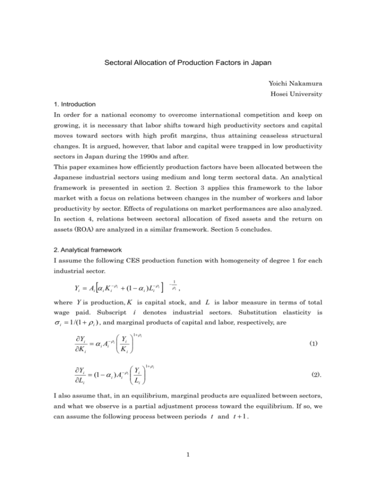
Sectoral Allocation of Production Factors in Japan
Yoichi Nakamura
Hosei University
1. Introduction
In order for a national economy to overcome international competition and keep on
growing, it is necessary that labor shifts toward high productivity sectors and capital
moves toward sectors with high profit margins, thus attaining ceaseless structural
changes. It is argued, however, that labor and capital were trapped in low productivity
sectors in Japan during the 1990s and after.
This paper examines how efficiently production factors have been allocated between the
Japanese industrial sectors using medium and long term sectoral data. An analytical
framework is presented in section 2. Section 3 applies this framework to the labor
market with a focus on relations between changes in the number of workers and labor
productivity by sector. Effects of regulations on market performances are also analyzed.
In section 4, relations between sectoral allocation of fixed assets and the return on
assets (ROA) are analyzed in a similar framework. Section 5 concludes.
2. Analytical framework
I assume the following CES production function with homogeneity of degree 1 for each
industrial sector.
[
Yi = Ai α i K i− ρi + (1 − α i ) L−i ρi
]
−
1
ρi
,
where Y is production, K is capital stock, and L is labor measure in terms of total
wage paid. Subscript
i denotes industrial sectors. Substitution elasticity is
σ i = 1 /(1 + ρ i ) , and marginal products of capital and labor, respectively, are
Y
∂Yi
= α i Ai− ρi  i
∂K i
 Ki



1+ ρ i
Y
∂Yi
= (1 − α i ) Ai− ρ i  i
∂Li
 Li
(1)



1+ ρ i
(2).
I also assume that, in an equilibrium, marginal products are equalized between sectors,
and what we observe is a partial adjustment process toward the equilibrium. If so, we
can assume the following process between periods t and t + 1 .
1
 ∂Y
 ∂Yi ,t +1 
 = log i ,t
log
 ∂K

 ∂K
 i ,t
 i ,t +1 
 ∂Y
 ∂Yi ,t +1 
 = log i ,t
log
 ∂L

 ∂L
 i ,t
 i ,t +1 


∂Y 
 + θ K  µ K − i ,t 

∂K i ,t 




∂Y 
 + θ L  µ L − i ,t 

∂Li ,t 


(3)
(4)
µ K and µ L above are the median marginal products of capital and labor through all
sectors and assumed to be constant. Substituting (1) and (2) into (3) and (4),
 Yi ,t +1 
 K i ,t +1 
∂Yi ,t

 = Z K' ,i + θ K' ,i
log
+ log
 Y 
 K 
K
∂
i ,t
 i ,t 
 i ,t 
(5)

Y
 Li ,t +1 
∂Y
 = Z L' ,i + θ L' ,i i ,t + log i ,t +1 
log
 Y 
 L 
∂Li ,t
 i ,t 
 i ,t 
(6)
where Z K' ,i = θ K µ K /(1 + ρ i ) , θ K' ,i = θ K /(1 + ρ i ) , Z L' ,i = θ L µ L /(1 + ρ i ) , θ L' ,i = θ L /(1 + ρ i ) .
Equations (5) and (6) show that changes in capital and labor depend on those in
production and marginal products. Marginal products are related to productivity by (1)
and (2).
3. Sectoral allocation of labor
I first examine relations between the number of employees and marginal product of
labor by sector. Unit labor cost1 is used as a measure of labor productivity in wage unit.
All data are from Annual Report on System of National Accounts (Cabinet Office). Data
from 1955 to 1998 are based on 68 SNA, and those from 1990 to 2000 are based on 93
SNA. This difference is not important because these data are converted into rates of
change during five-year periods.
The entire period of 1960 to 2000 is divided into 8 five-year periods, and the industry is
broken down into 19 sectors 2 . The data are pooled, and the following equation is
estimated for the entire periods and 6 sub-periods.
EMP = α + β ⋅ ULC + γ ⋅ OUTPUT
(7)
where EMP and OUTPUT are rates of changes in employees and real output (first
order difference in logarithm) in five-year periods (1960-65,1965-70,----), ULC is unit
labor cost in the first year of each period, which is divided (in order to normalize for
large differences between sectors) by its value five years before.
The presence of regulations on entry, exit and pricing may undermine ability of the
2
labor market to efficiently allocate the total labor between sectors. I introduce a dummy
variable representing scope and intensity of regulations, D . D is set at the number of
government committee reports in which a need for deregulation has been pointed out.
Since the finance and insurance sector, for instance, has been picked up as an industry
where deregulation is required by all of the three committees in Annex Table, D for
the sector is 3. Equation (7) is extended as,
EMP = α + ( β 1 + β 2 ⋅ D)ULC + γ ⋅ OUTPUT
(8)
Tables 1 and 2 show the estimation results of (7) and (8). As is shown in Table 1, a
negative effect of higher unit labor cost on increase in employment is significant. This is
more pronounced in the first 20 years (1960-80).
In the second 20-year period, however,
significance is lost. In the 1990s, the sign of the parameter on ULC is reversed. These
results suggest that in the era of rapid growth and structural adjustment of the 1960s
and 1970s, changes in productivity dictated labor allocation between industrial sectors
in Japan. In and after the 1980s, however, the Japanese labor market performed
differently.
3
Table 2 shows that the regulation dummy is significant. The parameter on ULC is
estimated at -0.1126. In the case of a sector for which D =3, this parameter reduces to
-0.0591. This suggests that the speed of adjustment based on unit labor cost was almost
half in heavily regulated sectors. The absolute values of the parameters are large in the
estimation results for the 70s, which include the period of industrial adjustment after
the oil shocks, implying that there was intensive reallocation of labor based on
productivity. The speed of reallocation, however, varied substantially between sectors
due to differences in intensity of regulation.
4. Sectoral allocation of capital stock
Next I turn to allocation of capital stock between sectors. Net fixed asset by sector at
current prices compiled by Japan Center for Economic Research, and operating surplus
in SNA are used. Data are available for the 1970-2000 period, which is divided into 6
five-year sub-periods. Letting ASSET and OUTPUT − N be first-order differences in
logarithm of net fixed asset and output in current prices, respectively, and ROA be the
ratio of operating surplus to net fixed asset in the first year of each five-year sub-period,
the following equation is estimated.
ASSET = α + β ⋅ ROA + γ ⋅ OUTPUT − N
(9)
An extended version including the regulation dummy is also estimated.
ASSET = α + ( β 1 + β 2 ⋅ D) ROA + γ ⋅ OUTPUT − N
Table 3 shows that, for the entire period, parameters on both
(10)
ROA
and
OUTPUT − N are significant, and capital stock of high-ROA sectors tended to grow
faster. Results for 3 sub-periods suggest that, while parameters obtained for the 1970s
4
are positive and significant, those for the 1980s lose significance. In the 1990s,
parameters turn to negative, albeit insignificant.
Table 4 shows that inclusion of the dummy variable improves fitness and reliability. The
parameter on the regulation dummy for the entire period is negative implying that
regulations disturbed resource allocation by market forces. Since the parameter on the
regulation dummy is about one third of that on ROA in absolute terms, effects of ROA
on capital allocation are almost canceled for the sectors with D =3, such as ‘finance and
insurance’ and ‘transportation and communication’. Estimation results for 3 sub-periods
are also improved. Parameter on the regulation dummy is negative and significant at
the 10 % level for the 1980s and the 1990s.
5. Concluding remarks
It is observed that there were relative increases in labor in the sectors with improving
productivity, and those in capital stock where rate of return was high in the 1970s. This
period, during which two oil shocks took place, saw substantial changes in relative price
structures, and many ‘structurally depressed industries’ emerged. Structural
adjustment carried out in Japan was highly evaluated in light of ongoing global
structural adjustment. The above findings imply that the structural adjustment in
Japan during the period was of a type which exploited resource allocation ability of the
market. And this may have been behind Japan’s overwhelming international
competitiveness in the 1980s. It is also observed that regulations had significant
5
negative effects on the factor allocation by market forces during the 1970s.
In the 1980-2000 period, factor allocation in Japan became less consistent with labor
productivity and return on capital. Asset bubbles and extreme labor shortage may
account for reduced consistency in the 1980s. Overall stagnation and financial crises in
the 1990s may have hindered structural changes. The malfunctioning of factor
allocation must have been one of the factors accounting for protracted economic
difficulties or ‘lost decade’ in Japan after 1990.
1
Defined as compensation of employees / (number of employees ¯ real output).
2
For sectoral break down, see Appendix Table.
6
References
Floystad, G., “Distortions in the Factor market: An Empirical Investigation,” Review of
Economics and Statistics, Vol.57, No.2 (May 1975), 200-213
Douugherty, C. and M. Selowsky, “Measuring the Effects of the Misallocation of
Labour,” Review of Economics and Statistics, Vol.55, No.3 (Aug. 1973), 386-390
Ulman, L., “Labor Mobility and the Industrial Wage Structure in the Postwar United
States,” Quarterly Journal of Economics, Vol.79, Issue 1 (Feb. 1965), 73-97
7