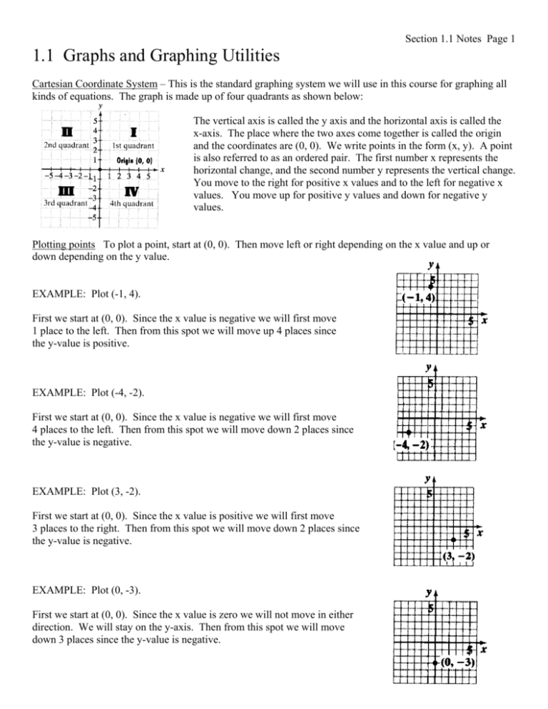
Section 1.1 Notes Page 1
1.1 Graphs and Graphing Utilities
Cartesian Coordinate System – This is the standard graphing system we will use in this course for graphing all
kinds of equations. The graph is made up of four quadrants as shown below:
The vertical axis is called the y axis and the horizontal axis is called the
x-axis. The place where the two axes come together is called the origin
and the coordinates are (0, 0). We write points in the form (x, y). A point
is also referred to as an ordered pair. The first number x represents the
horizontal change, and the second number y represents the vertical change.
You move to the right for positive x values and to the left for negative x
values. You move up for positive y values and down for negative y
values.
Plotting points To plot a point, start at (0, 0). Then move left or right depending on the x value and up or
down depending on the y value.
EXAMPLE: Plot (-1, 4).
First we start at (0, 0). Since the x value is negative we will first move
1 place to the left. Then from this spot we will move up 4 places since
the y-value is positive.
EXAMPLE: Plot (-4, -2).
First we start at (0, 0). Since the x value is negative we will first move
4 places to the left. Then from this spot we will move down 2 places since
the y-value is negative.
EXAMPLE: Plot (3, -2).
First we start at (0, 0). Since the x value is positive we will first move
3 places to the right. Then from this spot we will move down 2 places since
the y-value is negative.
EXAMPLE: Plot (0, -3).
First we start at (0, 0). Since the x value is zero we will not move in either
direction. We will stay on the y-axis. Then from this spot we will move
down 3 places since the y-value is negative.
Section 1.1 Notes Page 2
Graphing Equations by Making Tables and Plotting Points
The equations we are graphing in this section will be done by making a table of values and then plotting the
resulting points. Usually the question will tell you which values to use for x; otherwise use whichever values
for x you want. You should plot negatives, positives, and the zero. Later in this course we will learn how to
graph these without making tables.
EXAMPLE: Graph the equation y  2  x  1 . Let x = -3, -2, -1, 0, 1, 2, 3. Then indicate the intercepts.
It doesn’t matter if you’ve never graphed an absolute value before. We plot this one the same way we plot
lines. First we need to set up a table like this:
x
y  2  x 1
(x, y)
-3
-2
-1
0
1
2
3
Now what we do is plug in the x value into the equation y  2  x  1 . Then we write our answer as an
ordered pair as show below. Remember that absolute values always return a positive value. For example
5  5.
x
y  2  x 1
(x, y)
-3
y  2  (3)  1  2   4  2  4  2
(-3, -2)
-2
y  2  ( 2)  1  2   3  2  3  1
(-2, -1)
-1
y  2  (1)  1  2   2  2  2  0
(-1, 0)
0
y  2  ( 0)  1  2   1  2  1  1
(0, 1)
1
y  2  (1)  1  2  0  2  0  2
(1, 2)
2
y  2  ( 2)  1  2  1  2  1  1
(2, 1)
3
y  2  (3)  1  2  2  2  2  0
(3, 0)
To get the graph, just plot all these points. You will get this:
Let’s talk about the term intercepts. This is where the graph
crosses either the vertical or horizontal axis. Where ever the graph
crosses the vertical axis is called the y-intercept. Where ever
the graph crosses the horizontal axis is called the x-intercept. The
problem asked us to identify the intercepts. This means we need
to read them off our graph. For the y-intercept, this point would be
(0, 1). There are two places where it crosses the horizontal axis, and
this occurs at (-1, 0) and (3, 0).
Section 1.1 Notes Page 3
EXAMPLE: Graph the equation y  x  4 . Let x = -3, -2, -1, 0, 1, 2, 3. Then indicate the intercepts.
2
It doesn’t matter if you’ve never graphed a quadratic equation before. We plot this one the same way we plot
lines. First we need to set up a table like this:
x
y  x2  4
(x, y)
-3
-2
-1
0
1
2
3
Now what we do is plug in the x value into the equation y  x 2  4 . Then we write our answer as an ordered
pair as show below. Remember that a negative number raised to an even power is positive. For example
(5) 2  (5)(5)  25 .
x
y  x2  4
(x, y)
-3
y  (3) 2  4  9  4  5
(-3, 5)
-2
y  (2) 2  4  4  4  0
(-2, 0)
-1
y  (1) 2  4  1  4  3
(-1, -3)
0
y  (0) 2  4  0  4  4
(0, -4)
1
y  (1) 2  4  1  4  3
(1, -3)
2
y  (2) 2  4  4  4  0
(2, 0)
3
y  (3) 2  4  9  4  5
(3, 5)
To get the graph, just plot all these points. You will get this:
Now let’s identify the intercepts the same way we did it for the
previous problem. The y-intercept is where the graph crosses the
vertical axis. This point would be at (0, -4). There are two places
where it crosses the horizontal axis, and this occurs at (-2, 0) and (2, 0).
You can also write this as:  2, 0 .


Graphing Utilities
This book does some exercises where it wants you to set up viewing windows. Since I do not require graphing
calculators in this class, I am not requiring you to do these types of exercises. If you already have a graphing
calculator, you may use it for this class. Please ask me after class or in office hours if you have a specific
question on how to use your particular graphing calculator.