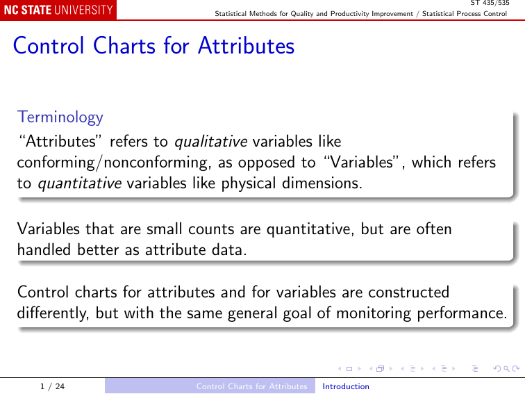
ST 435/535
Statistical Methods for Quality and Productivity Improvement / Statistical Process Control
Control Charts for Attributes
Terminology
“Attributes” refers to qualitative variables like
conforming/nonconforming, as opposed to “Variables”, which refers
to quantitative variables like physical dimensions.
Variables that are small counts are quantitative, but are often
handled better as attribute data.
Control charts for attributes and for variables are constructed
differently, but with the same general goal of monitoring performance.
1 / 24
Control Charts for Attributes
Introduction
ST 435/535
Statistical Methods for Quality and Productivity Improvement / Statistical Process Control
Examples
A glass container for a liquid product is classified as conforming
or nonconforming, based on the absence or presence of flaws.
The number of defects on a silicon wafer is counted.
Three different charts are used for data like these: the p chart, the c
chart, and the u chart.
2 / 24
Control Charts for Attributes
Introduction
ST 435/535
Statistical Methods for Quality and Productivity Improvement / Statistical Process Control
Control Chart for Fraction Nonconforming
Statistical framework
Suppose that items are produced, or services are provided, in a
sequence, and that each is classified as conforming or nonconforming.
Suppose that when the process is in control, successive items
indpendently have probability p of being nonconforming.
Then if a sample of n items has D nonconforming items, D has the
binomial distribution with parameters n and p:
D ∼ Bin(n, p).
3 / 24
Control Charts for Attributes
Control Chart for Fraction Nonconforming
ST 435/535
Statistical Methods for Quality and Productivity Improvement / Statistical Process Control
We estimate p by
D
,
n
and from the properties of Bin(n, p) we know that
p̂ =
E(p̂) = p
and
Var(p̂) =
p(1 − p)
.
n
We use these properties to construct a control chart called the p
chart.
4 / 24
Control Charts for Attributes
Control Chart for Fraction Nonconforming
ST 435/535
Statistical Methods for Quality and Productivity Improvement / Statistical Process Control
Development of the p chart
If p is known, plot each p̂ on a chart with a center line at p and
three-sigma control limits:
r
p(1 − p)
UCL = p + 3
n
Center line = p
r
p(1 − p)
.
LCL = p − 3
n
5 / 24
Control Charts for Attributes
Control Chart for Fraction Nonconforming
ST 435/535
Statistical Methods for Quality and Productivity Improvement / Statistical Process Control
If p is unknown, take m preliminary samples of size n.
Let
p̂i =
Di
,
n
i = 1, 2, . . . , m,
and
m
1 X
p̄ =
p̂i
m i=1
m
1 X
=
Di .
mn i=1
6 / 24
Control Charts for Attributes
Control Chart for Fraction Nonconforming
ST 435/535
Statistical Methods for Quality and Productivity Improvement / Statistical Process Control
Plot each p̂ on a chart with a center line at p̄ and three-sigma
control limits:
r
p̄(1 − p̄)
UCL = p̄ + 3
n
Center line = p̄
r
p̄(1 − p̄)
LCL = p̄ − 3
.
n
7 / 24
Control Charts for Attributes
Control Chart for Fraction Nonconforming
ST 435/535
Statistical Methods for Quality and Productivity Improvement / Statistical Process Control
Example: Orange juice cans
Cans are inspected for defective seals on side seam or bottom joint.
Development data: m = 30 samples of size n = 50, selected at 30
minute intervals.
In R:
cans <- read.csv("Data/Table-07-01-02.csv")
cansDev <- with(cans, Nonconforming[Phase == "I"])
summary(qcc(cansDev, type = "p", sizes = 50))
8 / 24
Control Charts for Attributes
Control Chart for Fraction Nonconforming
ST 435/535
Statistical Methods for Quality and Productivity Improvement / Statistical Process Control
Data points 15 and 23 are above the UCL; inspection reveals
assignable causes to both (new batch of cardboard, inexperienced
operator).
Recompute limits, excluding those points:
summary(qcc(cansDev[-c(15, 23)], type = "p", sizes = 50))
One more data point is above the new UCL, but no assignable cause
was found, and the process was declared in-control.
Note: Montgomery suggests including points 15 and 23 in the chart,
just leaving them out of the calculations; not currently possible in
qcc().
9 / 24
Control Charts for Attributes
Control Chart for Fraction Nonconforming
ST 435/535
Statistical Methods for Quality and Productivity Improvement / Statistical Process Control
21% nonconforming cans was not acceptable, so the equipment was
adjusted.
Using the chart for subsequent operations; 24 additional samples:
cansUse <- with(cans, Nonconforming[Phase == "II"])
summary(qcc(cansDev[-c(15, 23)], type = "p", sizes = 50,
newdata = cansUse, newsizes = 50))
The lengthy run below the center line and the one point below the
LCL indicate that the fraction nonconforming has been reduced.
The control limits were recomputed based on the later samples.
10 / 24
Control Charts for Attributes
Control Chart for Fraction Nonconforming
ST 435/535
Statistical Methods for Quality and Productivity Improvement / Statistical Process Control
The np chart
In some areas the convention is to chart the number nonconforming,
instead of the fraction nonconforming.
When the sample sizes are all equal, this is a trivial change:
summary(qcc(cansDev[-c(15, 23)], type = "np", sizes = 50,
newdata = cansUse, newsizes = 50))
11 / 24
Control Charts for Attributes
Control Chart for Fraction Nonconforming
ST 435/535
Statistical Methods for Quality and Productivity Improvement / Statistical Process Control
Unequal sample sizes
If the development data have sample sizes ni , i = 1, 2, . . . , m, we
estimate p by
Pm
Di
p̄ = Pi=1
m
i=1 ni
Three-sigma control limits vary by sample:
s
p̄(1 − p̄)
UCL = p̄ + 3
ni
Center line = p̄
s
LCL = p̄ − 3
12 / 24
p̄(1 − p̄)
.
ni
Control Charts for Attributes
Control Chart for Fraction Nonconforming
ST 435/535
Statistical Methods for Quality and Productivity Improvement / Statistical Process Control
Example: Erroneous purchase orders
Purchase orders issued by an aerospace company may not be correct.
Samples are based on weeks of operation, and different numbers of
POs are issued each week.
orders <- read.csv("Data/Table-07-04.csv")
summary(qcc(orders$Nonconforming, sizes = orders$Size,
type = "p"))
Other solutions are to use the average sample size (not
recommended) or the standardized chart, based on
p̂i − p
Zi = q
.
p(1−p)
ni
13 / 24
Control Charts for Attributes
Control Chart for Fraction Nonconforming
ST 435/535
Statistical Methods for Quality and Productivity Improvement / Statistical Process Control
Operating characteristics
The operating characteristic (OC) curve is a graph of the β-risk
against the actual fraction nonconforming.
For the orange juice cans:
oc.curves(qcc(cansDev, type = "p", sizes = 50))
The flat top means that small changes in p are hard to detect in a
single sample, but the ARL1 = 1/β may be acceptable.
14 / 24
Control Charts for Attributes
Control Chart for Fraction Nonconforming
ST 435/535
Statistical Methods for Quality and Productivity Improvement / Statistical Process Control
Control Chart for Nonconformities
In some contexts, a product or a service as a whole may be classified
as nonconforming if it contains too many individual nonconformities.
For example: flaws in the paint of a car; one or two may be
acceptable, but more than two is not.
15 / 24
Control Charts for Attributes
Control Chart for Nonconformities
ST 435/535
Statistical Methods for Quality and Productivity Improvement / Statistical Process Control
Statistical framework
The simplest distribution for counted data like these is the Poisson
distribution:
e −c c x
P(X = x) =
,
x!
where X is the number of nonconformities and c is the parameter of
the distribution.
Since
E(X ) = Var(X ) = c,
three-sigma limits for known c are:
√
UCL = c + 3 c
Center line = c
√
LCL = c − 3 c.
16 / 24
Control Charts for Attributes
Control Chart for Nonconformities
ST 435/535
Statistical Methods for Quality and Productivity Improvement / Statistical Process Control
When c is unknown, m preliminary counts x1 , x2 , . . . , xm are made,
and c is estimated by
m
1 X
c̄ = x̄ =
xi .
m i=1
Three-sigma limits for unknown c are then:
√
UCL = c̄ + 3 c̄
Center line = c̄
√
LCL = c̄ − 3 c̄.
This is the c control chart.
17 / 24
Control Charts for Attributes
Control Chart for Nonconformities
ST 435/535
Statistical Methods for Quality and Productivity Improvement / Statistical Process Control
Example: printed circuit boards
The inspection unit is a sample of 100 boards, and X is the number
of nonconformities in the sample. Preliminary counts are for m = 26
samples
In R:
boards <- read.csv("Data/Table-07-07-08.csv")
boardsDev <- with(boards, Nonconformities[Phase == "I"])
summary(qcc(boardsDev, type = "c"))
18 / 24
Control Charts for Attributes
Control Chart for Nonconformities
ST 435/535
Statistical Methods for Quality and Productivity Improvement / Statistical Process Control
Two data points are outside the control limits, and investigation
showed that both have assignable causes (inexperienced inspector,
problem with wave soldering), so they are omitted:
summary(qcc(boardsDev[-c(6, 20)], type = "c"))
Remaining points are all within limits, so these limits are used for
subsequent operations:
summary(qcc(boardsDev[-c(6, 20)], type = "c",
newdata = boardsUse))
19 / 24
Control Charts for Attributes
Control Chart for Nonconformities
ST 435/535
Statistical Methods for Quality and Productivity Improvement / Statistical Process Control
Further analysis
Number of nonconformities is high, so types of nonconformity were
shown in a Pareto chart:
boardsPareto <- read.csv("Data/Figure-07-14.csv")
Frequency <- boardsPareto$Frequency
names(Frequency) <- boardsPareto$Defect.Code
pareto.chart(Frequency)
The chart shows that most of the nonconformities were of just two
types, both related to soldering.
20 / 24
Control Charts for Attributes
Control Chart for Nonconformities
ST 435/535
Statistical Methods for Quality and Productivity Improvement / Statistical Process Control
Unequal sample sizes
In some situations, nonconformities are counted for different numbers
of sampling units in each sample.
If Xi is the count for ni sampling units, and the average number of
defects per sampling unit is u, then Xi ∼ Poisson(ni u), and
E(Xi ) = Var(Ui ) = ni u.
If these counts xi are plotted on a c chart, the center line and the
control lines all vary from sample to sample; qcc() refuses to make
such a chart.
21 / 24
Control Charts for Attributes
Control Chart for Nonconformities
ST 435/535
Statistical Methods for Quality and Productivity Improvement / Statistical Process Control
Instead, let
Ui =
Xi
,
ni
so that
E(Ui ) = u,
Var(Ui ) =
u
.
ni
These may be plotted on a u chart with three-sigma limits, which for
known u are:
r
u
UCL = u + 3
ni
Center line = u
r
u
LCL = u − 3
.
ni
22 / 24
Control Charts for Attributes
Control Chart for Nonconformities
ST 435/535
Statistical Methods for Quality and Productivity Improvement / Statistical Process Control
For unknown u, estimate u from m preliminary samples:
Pm
Pm
xi
ni ui
i=1
ū = Pm
= Pi=1
.
m
i=1 ni
i=1 ni
The three-sigma limits become
r
UCL = ū + 3
ū
ni
Center line = ū
r
ū
LCL = ū − 3
.
ni
23 / 24
Control Charts for Attributes
Control Chart for Nonconformities
ST 435/535
Statistical Methods for Quality and Productivity Improvement / Statistical Process Control
Example: Dyed cloth
Dyed cloth is inspected for defects per 50 square meters. Ten rolls
are inspected, with varying areas.
cloth <- read.csv("Data/Table-07-12.csv")
summary(qcc(cloth$Nonconformities, type = "u",
sizes = cloth$Square.Meters / 50))
The u chart may also be used with equal sample sizes, when it is
desired to report results on a per-unit basis instead of a per-sample
basis.
24 / 24
Control Charts for Attributes
Control Chart for Nonconformities