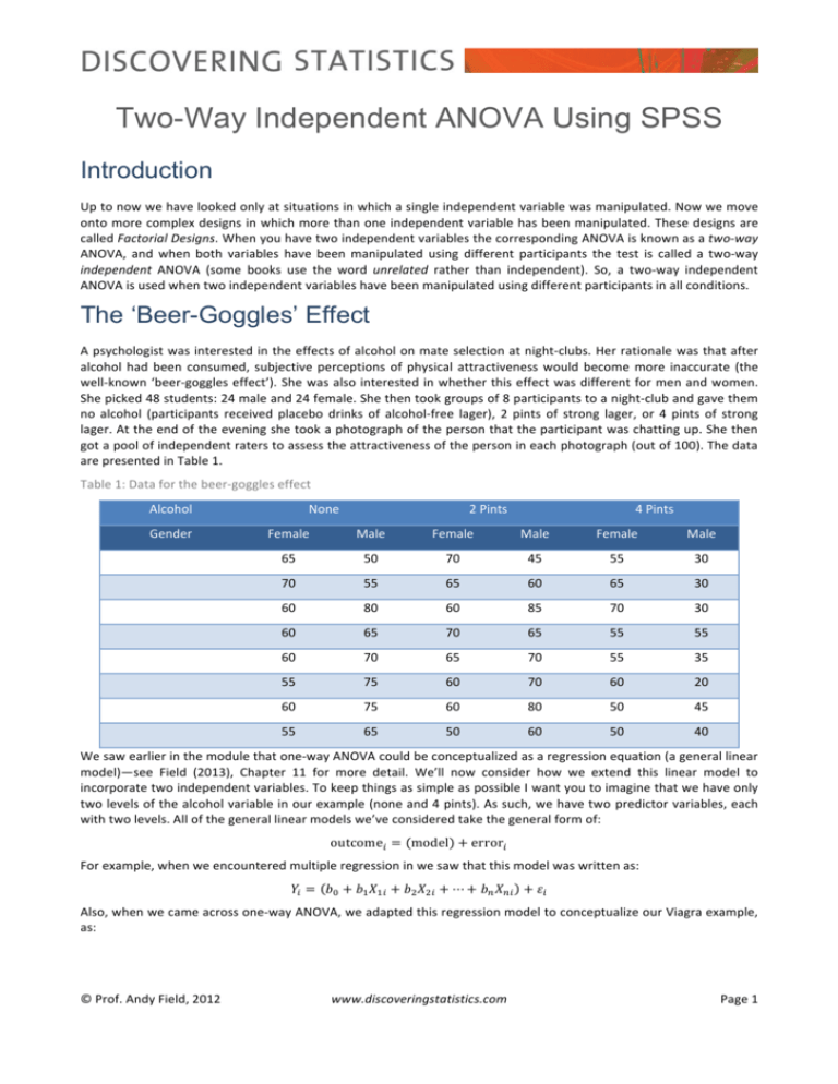
Two-Way Independent ANOVA Using SPSS
Introduction
Up to now we have looked only at situations in which a single independent variable was manipulated. Now we move onto more complex designs in which more than one independent variable has been manipulated. These designs are called Factorial Designs. When you have two independent variables the corresponding ANOVA is known as a two-­‐way ANOVA, and when both variables have been manipulated using different participants the test is called a two-­‐way independent ANOVA (some books use the word unrelated rather than independent). So, a two-­‐way independent ANOVA is used when two independent variables have been manipulated using different participants in all conditions. The ‘Beer-Goggles’ Effect
A psychologist was interested in the effects of alcohol on mate selection at night-­‐clubs. Her rationale was that after alcohol had been consumed, subjective perceptions of physical attractiveness would become more inaccurate (the well-­‐known ‘beer-­‐goggles effect’). She was also interested in whether this effect was different for men and women. She picked 48 students: 24 male and 24 female. She then took groups of 8 participants to a night-­‐club and gave them no alcohol (participants received placebo drinks of alcohol-­‐free lager), 2 pints of strong lager, or 4 pints of strong lager. At the end of the evening she took a photograph of the person that the participant was chatting up. She then got a pool of independent raters to assess the attractiveness of the person in each photograph (out of 100). The data are presented in Table 1. Table 1: Data for the beer-­‐goggles effect Alcohol None 2 Pints 4 Pints Gender Female Male Female Male Female Male 65 50 70 45 55 30 70 55 65 60 65 30 60 80 60 85 70 30 60 65 70 65 55 55 60 70 65 70 55 35 55 75 60 70 60 20 60 75 60 80 50 45 55 65 50 60 50 40 We saw earlier in the module that one-­‐way ANOVA could be conceptualized as a regression equation (a general linear model)—see Field (2013), Chapter 11 for more detail. We’ll now consider how we extend this linear model to incorporate two independent variables. To keep things as simple as possible I want you to imagine that we have only two levels of the alcohol variable in our example (none and 4 pints). As such, we have two predictor variables, each with two levels. All of the general linear models we’ve considered take the general form of: outcome! = model + error!
For example, when we encountered multiple regression in we saw that this model was written as: 𝑌𝑌! = 𝑏𝑏! + 𝑏𝑏! 𝑋𝑋!! + 𝑏𝑏! 𝑋𝑋!! + ⋯ + 𝑏𝑏! 𝑋𝑋!" + 𝜀𝜀!
Also, when we came across one-­‐way ANOVA, we adapted this regression model to conceptualize our Viagra example, as: © Prof. Andy Field, 2012 www.discoveringstatistics.com Page 1 Libido! = 𝑏𝑏! + 𝑏𝑏! high! + 𝑏𝑏! low! + 𝜀𝜀!
In this model, the High and Low variables were dummy variables (i.e., variables that can take only values of 0 or 1). In our current example, we have two variables: gender (male or female) and alcohol (none and 4 pints). We can code each of these with zeros and ones, for example, we could code gender as male = 0, female = 1, and we could code the alcohol variable as 0 = none, 1 = 4 pints. We could then directly copy the model we had in one-­‐way ANOVA: Attractiveness! = 𝑏𝑏! + 𝑏𝑏! Gender! + 𝑏𝑏! Alcohol! + 𝜀𝜀!
However, this model does not consider the interaction between gender and alcohol. If we want to include this term too, then the model simply extends to become (first expressed generally and then in terms of this specific example): Attractiveness! = 𝑏𝑏! + 𝑏𝑏! A ! + 𝑏𝑏! B! + 𝑏𝑏! AB! + 𝜀𝜀! Attractiveness! = 𝑏𝑏! + 𝑏𝑏! Gender! + 𝑏𝑏! Alcohol! + 𝑏𝑏! Interaction! + 𝜀𝜀! The question is: how do we code the interaction term? The interaction term represents the combined effect of alcohol and gender; to get any interaction term you simply multiply the variables involved. This is why you see interaction terms written as gender × alcohol, because in regression terms the interaction variable literally is the two variables multiplied by each other. For more detail about how all of the coding works read Field (2013), Chapters 10 and 12. For the purpose of this exercise all I really want you to understand is that (1) we’re still fitting a linear model; (2) SPSS will code your predictors (independent variables) using the dummy coding that we have discussed before; and (3) we include an interaction term, which is coded by multiplying the dummy codes for any of the predictors involved in the interaction. Two-Way Independent ANOVA Using SPSS
Inputting Data
→ Levels of between group variables go in a single column of the SPSS data editor. Applying the rule above to the data we have here we are going to need to create 2 different coding variables (seeField, 2013, Chapter 3) in the data editor. These columns will represent gender and alcohol consumption. So, create a variable called Gender in the data editor and activate the labels dialog box. You should define value labels to represent the two genders. We have had a lot of experience with coding values, so you should be fairly happy about assigning numerical codes to different groups. I recommend using the code Male = 0, and Female = 1. Once you have done this, you can enter a code of zero or one in this column indicating to which group the participant belonged. Create a second variable called Alcohol and assign group codes by using the labels dialog box. I suggest that you code this variable with three values: Placebo (no Alcohol) = 1, 2 Pints = 2, and 4 pints = 3. You can now enter 1, 2 or 3 into this column to represent the amount of alcohol consumed by the participant. Remember that if you turn the value labels option on ( ) you will see text in the data editor rather than the numerical codes. Now, the way this coding works is as follows: Gender Alcohol Participant was .. 0 1 Male who consumed no alcohol 0 2 Male who consumed 2 pints 0 3 Male who consumed 4 pints 1 1 Female who consumed no alcohol 1 2 Female who consumed 2 pints 1 3 Female who consumed 4 pints © Prof. Andy Field, 2012 www.discoveringstatistics.com Page 2 Once you have created the two coding variables, you can create a third variable in which to place the values of the dependent variable. Call this variable attract and use the labels option to give it the fuller name of ‘Attractiveness of Date’. In this example, there are two independent variables and different participants were used in each condition: hence, we can use the general factorial ANOVA procedure in SPSS. This procedure is designed for analysing between-­‐
group factorial designs. → Enter the data into SPSS. → Save the data onto a disk in a file called BeerGoggles.sav. → Plot an error bar graph of the mean attractiveness of mates across the different levels of alcohol. → Plot an error bar graph of the mean attractiveness of mates selected by males and females. The Main Dialog Box
To access the main dialog box use the file path . The resulting dialog box is shown in Figure 1. First, select the dependent variable Attractiveness from the variables list on the left-­‐hand side of the dialog box and drag it to the space labelled Dependent Variable or click on . In the space labelled Fixed Factor(s) we need to place any independent variables relevant to the analysis. Select Alcohol and Gender in the variables list (these variables can be selected simultaneously by holding down Ctrl while clicking on the variables) and drag them to the Fixed Factor(s) box (or click on ). There are various options available to us, we only need worry about the ones covered in this handout (anyone interested in further options should read my 2013 textbook, chapter 13). Figure 1: Main dialog box for univariate ANOVA Simple and horrible looking graphs of Interactions
Click on to access the dialog box in Figure 2. The plots dialog box allows you to select line graphs of your data and these graphs are very useful for interpreting interaction effects (however, really we should plot graphs of the means before the data are analysed). We have only two independent variables, and the most useful plot is one that shows the interaction between these variables (the plot that displays levels of one independent variable against the other). In this case, the interaction graph will help us to interpret the combined effect of gender and alcohol consumption. Select Alcohol from the variables list on the left-­‐hand side of the dialog box and drag it to the space labelled Horizontal Axis (or click on ). In the space labelled Separate Lines place the remaining independent variable, Gender. It doesn’t matter which way round the variables are plotted; you should use your discretion as to which way produces the most sensible graph. When you have moved the two independent variables to the appropriate box, click on and this plot will be added to the list at the bottom of the box. You can plot a whole © Prof. Andy Field, 2012 www.discoveringstatistics.com Page 3 variety of graphs, and if you had a third independent variable, you have the option of plotting different graphs for each level of that third variable by specifying a variable under the heading Separate Plots. When you have finished specifying graphs, click on to return to the main dialog box. Figure 2: Specifying plots Post Hoc Tests
The post hoc tests dialog box is obtained by clicking on in the main dialog box (Figure 3). The variable Gender has only two levels and so we don’t need to select post hoc tests for that variable (because any significant effects can reflect only the difference between males and females). However, there were three levels of the Alcohol variable (no alcohol, 2 pints and 4 pints); hence we can conduct post hoc tests (although remember that normally you would conduct contrasts or post hoc tests, not both). First, you should select the variable Alcohol from the box labelled Factors and transfer it to the box labelled Post Hoc Tests for. My recommendations for which post hoc procedures to use are in last weeks handout (and I don’t want to repeat myself). Suffice to say you should select the ones in Figure 3! Click on to return to the main dialog box. Figure 3: Dialog box for post hoc tests © Prof. Andy Field, 2012 www.discoveringstatistics.com Page 4 Options
Click on to activate the dialog box in Figure 4. The options for factorial ANOVA are fairly straightforward. First you can ask for some descriptive statistics, which will display a table of the means and standard deviations. This is a useful option to select because it assists in interpreting the final results. You can select the homogeneity of variance tests (see your handout on bias). Once these options have been selected click on to return to the main dialog box. Figure 4: Dialog box for options Bootstrapping
As with any ANOVA, the main dialog box contains the button, which enables you to select bootstrapped confidence intervals for the estimated marginal means, descriptives and post hoc tests, but not the main F test. The main use of these is if you plan to look at the post hoc tests, which we are, so select the options in Figure 5. Once these options have been selected click on to return to the main dialog box, then click on run the analysis. Figure 5: Bootstrap dialog box © Prof. Andy Field, 2012 www.discoveringstatistics.com Page 5 Output from Factorial ANOVA
Output for the Preliminary Analysis
Output 1 shows a table of descriptive statistics produced because we asked for descriptives in the options dialog box (see Figure 4) (if you don’t ask for bootstrapping this table will be a bit more straightforward); it displays the means, standard deviations, confidence intervals and number of participants in all conditions of the experiment. So, for example, we can see that in the placebo condition, Males typically chatted up a female that was rated at about 67% on the attractiveness scale and the bootstrapped confidence interval for the mean ranges from 59.54 to 73.33. Females on the other hand selected a mate that was rated as 61% on that scale and the bootstrapped confidence interval for the mean ranges from 57.50 to 64.50. Note that the confidence intervals for the two groups overlap, implying that they might be from the same population. These means will be useful in interpreting the direction of any effects that emerge in the analysis. Output 1 © Prof. Andy Field, 2012 www.discoveringstatistics.com Page 6 Effect Sizes (Cohen’s d)
We could use the means in Output 1 to compute effect sizes. For example, we might look at the effect of gender within each alcohol condition. Remember from earlier in the module that Cohen’s d is the difference between two means divided by some estimate of the standard deviation of those means: 𝑑𝑑 =
𝑋𝑋! − 𝑋𝑋!
𝑠𝑠
The s can be the standard deviation of the control group, or a pooled estimate (see the handout on One-­‐way ANOVA, or Field, 2013, chapter 2). If we’re looking at gender there isn't a logical control group so we should use a pooled estimate. Have a go at calculating these effect sizes. The results are in Table 2. Table 2: Cohen’s d for the effect of gender within each alcohol group Comparison Sp dpooled No Pints (Male vs. Female) 8.10 0.77 2 Pints (Male vs. Female) 9.99 0.44 4 Pints (Male vs. Female) 9.15 −2.39 Levene’s Test
Output 2 shows the results of Levene’s test (see handouts on bias and one-­‐way independent ANOVA). You should recall that a non-­‐significant result (as found here) is indicative of the homogeneity of variance assumption being met. You should also bear in mind the various discussions we’ve had about being cautious in using tests such as Levene’s. Output 2 The Main ANOVA Table
Output 3 is the most important part of the output because it tells us whether any of the independent variables have had an effect. The important things to look at in the table are the significance values of the independent variables. The first thing to notice is that there is a significant effect of alcohol (because the significance value is less than .05). The F ratio is highly significant indicating that the amount of alcohol consumed significantly effected who the participant would try to chat up. This effect means that overall, when we ignore whether the participant was male or female, the amount of alcohol influenced their mate selection. The best way to see what this means is to look at the bar chart that you (should) have plotted of the average mark for each level of alcohol (ignoring gender completely) — this shows the means in Output 1. © Prof. Andy Field, 2012 www.discoveringstatistics.com Page 7 Output 3 This effect should be reported as: → There was a significant main effect of the amount of alcohol consumed at the night-­‐club, on the attractiveness of the mate that was selected, F(2, 42) = 20.07, p < .001. Figure 6 shows that when you ignore gender the overall attractiveness of the selected mate is very similar when no alcohol has been drunk, and when 2 pints were drunk (the means of these groups are approximately equal). Hence, this significant main effect is likely to reflect the drop in the attractiveness of the selected mates when 4 pints has been drunk. This finding seems to indicate that a person is willing to accept a less attractive mate after 4 pints. Figure 6: Graph showing the main effect of alcohol. Output 3also reports the main effect of gender. This time the F ratio is not significant (p = .161, which is larger than .05). This effect means that overall, when we ignore how much alcohol had been drunk, the gender of the participant did not influence the attractiveness of the partner that the participant selected. In other words, other things being equal, males and females selected equally attractive mates. The meaning of this main effect can be seen in the error bar chart you were asked to plot at the beginning of this handout: it shows the average attractiveness of mates for men and women (ignoring how much alcohol had been consumed). This effect should be reported as: → There was a nonsignificant main effect of gender on the attractiveness of selected mates, F(1, 42) = 2.03, p = .161. © Prof. Andy Field, 2012 www.discoveringstatistics.com Page 8 Figure 7: Graph to show the effect of gender on mate selection Figure 7 shows that the average attractiveness of the partners of male and female participants was fairly similar (the means are different by only 4%). Therefore, this nonsignificant effect reflects the fact that the mean attractiveness was similar. We can conclude from this that, ceteris paribus, men and women chose equally attractive partners. Finally, Output 3 tells us about the interaction between the effect of gender and the effect of alcohol. The F value is highly significant (because the p-­‐value is less than .05). This effect should be reported as: → There was a significant interaction between the amount of alcohol consumed and the gender of the person selecting a mate, on the attractiveness of the partner selected, F(2, 42) = 11.91, p < .001. Figure 8: Graph of the interaction effect © Prof. Andy Field, 2012 www.discoveringstatistics.com Page 9 What this actually means though, is that the effect of alcohol on mate selection was different for male participants than it was for females. The SPSS output includes a plot that we asked for (see Figure 2) which tells us something about the nature of this interaction effect. The graph that SPSS produces looks horrible and scales the y-­‐axis such that the interaction effect is maximised. This, as we have seen in previous weeks is bad practice. Figure 8 shows a better graph that I edited to look niceJ. Figure 8 shows that for women, alcohol has very little effect: the attractiveness of their selected partners is quite stable across the three conditions (as shown by the near-­‐horizontal line). However, for the men, the attractiveness of their partners is stable when only a small amount has been drunk, but rapidly declines when more is drunk. A significant interaction effect is usually shown by non-­‐parallel lines on a graph like this one. In this particular graph the lines actually cross, which indicates a fairly large interaction between independent variables. The interaction effect tells us that alcohol has little effect on mate selection until 4 pints have been drunk and that the effect of alcohol is prevalent only in male participants (so, basically, women maintain high standards in their mate selection regardless of alcohol, whereas men have a few beers and go for anything on legs!). One interesting point that these data demonstrate is that we concluded earlier that alcohol significantly affected how attractive a mate was selected (the alcohol main effect); however, the interaction effect tells us that this is true only in males (females are unaffected). This shows how misleading main effects can be: it is usually the interactions between variables that are most interesting in a factorial design. Post Hoc Analysis
The Bonferroni post hoc tests (Output 4) break down the main effect of alcohol and can be interpreted as if a one-­‐way ANOVA had been conducted on the Alcohol variable (i.e., the reported effects for alcohol are collapsed with regard to gender). The tests show (both by the significance and whether the bootstrap confidence intervals cross zero) that when participants had drunk no alcohol or 2 pints of alcohol, they selected equally attractive mates, p = 1.00 (this is the maximum that p can be which reflects the fact that the means are almost identical). However, after 4 pints had been consumed, participants selected significantly less attractive mates than after both 2 pints (p < .001) and no alcohol (p < .001). It is interesting to note that the mean attractiveness of partners after no alcohol and 2 pints were so similar that the probability of the obtained difference between those means is 1 (i.e. completely probable!). The R-­‐
E-­‐G-­‐W-­‐Q test (Output 5) confirms that the means of the placebo and 2 pint conditions were equal whereas the mean of the 4-­‐pint group was different. It should be noted that these post hoc tests ignore the interactive effect of gender and alcohol. Output 4 © Prof. Andy Field, 2012 www.discoveringstatistics.com Page 10 Output 5 These post hoc tests should be reported as: → Confidence intervals are based on 1000 bootstrap samples. Bonferroni post hoc tests showed that the attractiveness of partners was similar after no alcohol and 2 pints, Mdiff = −0.94, 95% CI [−6.72, 5.23], p = 1; however, it was lower after 4 pints compared to none, Mdiff = 17.19, 95% CI [9.77, 25.61], p < .001 and significantly lower after 4 pints compared to 2, Mdiff = 18.13, 95% CI [10.40, 25.73], p < .001. Guided Example
Back in your week 1 handout on revising SPSS we came across an example based on Shackelford et al.’s (2000) study that looked at emotional reactions to infidelity (it’s in Cognition & Emotion, 14, 643-­‐659). The upshot is that men get homicidal and suicidal and women feel undesirable and insecure. Let’s imagine we did something similar: we took 24 men and 24 women and got their partners to tell them they had slept with someone else. We then took each person to a shooting gallery and gave them a gun and 100 bullets. For half of the men and women there was a human shaped target with a picture of their own face on it, and for the remainder there was a target with their partner’s face on it. They were left alone with each target for 5 minutes and the number of bullets used was measured. Table 3: Infidelity data Male Partner’s Face on the Target Their Own face on the Target Partner’s Face on the Target Their Own face on the Target 69 33 70 97 76 26 74 80 70 10 64 88 76 51 43 100 72 34 51 100 65 28 93 58 82 27 48 95 71 9 51 83 71 33 74 97 75 11 73 89 52 14 41 69 34 46 84 82 © Prof. Andy Field, 2012 Female www.discoveringstatistics.com Page 11 → Enter the data into SPSS. → Save the data onto a disk in a file called Infidelity.sav. → Plot two error bar graphs of the mean number of bullets across the different levels of gender and type of face on the target respectively. → Conduct a two-­‐way independent ANOVA to see whether the number of bullets used was affected by gender, the face on the target or their interaction. Your Answer: Your Answer: Your Answer: Your Answer: What are the independent variables and how many levels do they have? What is the dependent variable? Describe the assumption of homogeneity of variance. Has this assumption been met? (Quote relevant statistics in APA format). Report the main effect of gender in APA format. Is this effect significant and how would you interpret it? © Prof. Andy Field, 2012 www.discoveringstatistics.com Page 12 Your Answer: Your Answer: Report the main effect of ‘type of face on the target’ in APA format. Is this effect significant and how would you interpret it? Report the interaction effect between gender and ‘type of face on the target’ in APA format. Is this effect significant and how would you interpret it? Do the results support Shackelford et al.’s (2000) findings? Explain your answer. © Prof. Andy Field, 2012 www.discoveringstatistics.com Page 13 Your Answer: Task 1
People’s musical tastes tend to change as they get older: my parents, for example, after years of listening to relatively cool music when I was a kid, subsequently hit their mid-­‐forties and developed a worrying obsession with country and western music. This possibility worries me immensely because the future seems incredibly bleak if it is spent listening to Garth Brooks and thinking ‘oh boy, did I underestimate Garth’s immense talent when I was in my 20s’. So, I thought I’d do some research; I took two groups (age): young people (which I arbitrarily decided was under 40 years of age) and older people (above 40 years of age). I split each of these groups of 45 into three smaller groups of 15 and assigned them to listen to Fugazi, ABBA or Barf Grooks (music). I got each person to rate it (liking) on a scale ranging from −100 (I hate this foul music) through 0 (I am completely indifferent) to +100 (I love this music so much I’m going to explode). Table 4: Fugazi data Music Fugazi Age Young Old Young Barf Grooks Old Young Old 96 -­‐75 65 24 -­‐54 69 69 -­‐98 86 30 -­‐56 92 61 -­‐97 37 80 -­‐97 76 39 -­‐75 59 75 -­‐40 76 94 -­‐45 49 72 -­‐65 81 71 -­‐73 59 60 -­‐88 51 62 -­‐75 42 42 -­‐77 27 62 -­‐75 88 90 -­‐52 91 38 -­‐87 92 55 -­‐54 97 69 -­‐49 41 60 -­‐118 83 40 -­‐83 64 87 -­‐41 56 45 -­‐77 73 56 -­‐84 66 © Prof. Andy Field, 2012 Abba www.discoveringstatistics.com Page 14 86 -­‐75 66 54 -­‐66 122 93 -­‐98 73 74 -­‐77 62 68 -­‐97 68 40 -­‐103 65 → Enter the data into SPSS. → Save the data onto a disk in a file called Fugazi.sav. → Plot two error bar graphs of the mean liking across the different levels of age and type of music respectively . → Conduct a two-­‐way independent ANOVA to see whether liking ratings were affected by age, style of music or their interaction. → Answers can be found on the companion website of my book. Task 2
There are reports of increases in injuries related to playing Nintendo Wii (http://ow.ly/ceWPj). These injuries were attributed mainly to muscle and tendon strains. A researcher hypothesized that a stretching warm-­‐up before playing Wii would help lower injuries, and that athletes would be less susceptible to injuries because their regular activity makes them more flexible. She took 60 athletes and 60 non athletes (athlete), half of them played Wii and half watched others playing as a control (wii), and within these groups half did a 5 minute stretch routine before playing/watching whereas the other half did not (stretch). The outcome was a pain score out of 10 (where 0 is no pain, and 10 is severe pain) after playing for 4 hours (injury). The data are in the file Wii.sav (available from ) conduct a three-­‐way ANOVA to test whether athletes are less prone to injury, and whether the prevention program worked. Answers are available in the smart http://www.uk.sagepub.com/field4e/study/smartalex.htm Alex answers for Chapter 13 Multiple Choice Tests
Complete the multiple choice questions for Chapter 13 on the companion website to Field (2013): http://www.uk.sagepub.com/field4e/study/mcqs.htm. If you get any wrong, re-­‐read this handout (or Field, 2013, Chapter 13) and do them again until you get them all correct. Copyright Information
This handout contains material from: Field, A. P. (2013). Discovering statistics using SPSS: and sex and drugs and rock ‘n’ roll (4th Edition). London: Sage. This material is copyright Andy Field (2000, 2005, 2009, 2013). References
Field, A. P. (2013). Discovering statistics using IBM SPSS Statistics: And sex and drugs and rock 'n' roll (4th ed.). London: Sage. © Prof. Andy Field, 2012 www.discoveringstatistics.com Page 15