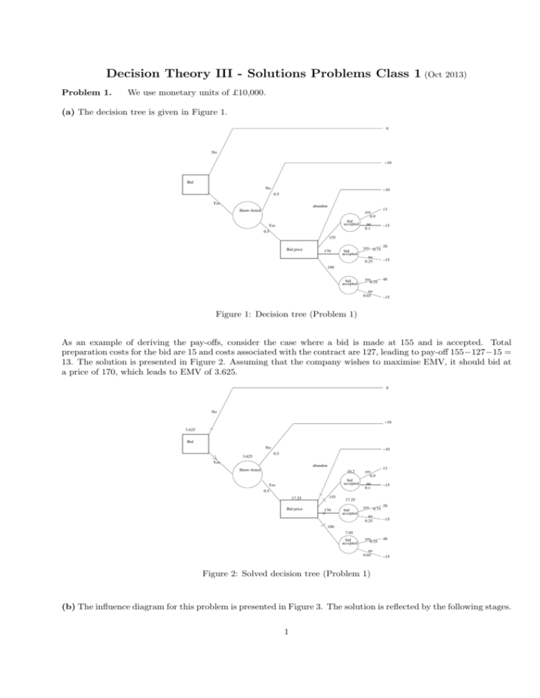
Decision Theory III - Solutions Problems Class 1 (Oct 2013)
Problem 1.
We use monetary units of £10,000.
(a) The decision tree is given in Figure 1.
0
No
−10
Bid
No
−10
0.5
Yes
abandon
Short−listed
yes
0.9
bid
accepted
Yes
0.5
no
0.1
13
−15
155
Bid price
170
bid
accepted
yes 0.75 28
no
0.25
−15
yes
0.35
48
190
bid
accepted
no
0.65
−15
Figure 1: Decision tree (Problem 1)
As an example of deriving the pay-offs, consider the case where a bid is made at 155 and is accepted. Total
preparation costs for the bid are 15 and costs associated with the contract are 127, leading to pay-off 155−127−15 =
13. The solution is presented in Figure 2. Assuming that the company wishes to maximise EMV, it should bid at
a price of 170, which leads to EMV of 3.625.
0
No
−10
3.625
Bid
No
3.625
−10
0.5
Yes
abandon
Short−listed
10.2
bid
accepted
Yes
0.5
17.25
Bid price
155
170
yes
0.9
no
0.1
13
−15
17.25
bid
accepted
yes 0.75 28
no
0.25
−15
yes
0.35
48
190
7.05
bid
accepted
no
0.65
−15
Figure 2: Solved decision tree (Problem 1)
(b) The influence diagram for this problem is presented in Figure 3. The solution is reflected by the following stages.
1
Short-listed
No
Yes
Yes
Bid accepted
No
Yes
Probability
0.5
0.125
0.375
Pay-off
-10
-15
28
Table 1: Risk profile of optimal solution (Problem 1)
First remove the ‘bid accepted’ node (as all parents already have direct links into the value node, no additonal
links are required; this also holds for the following steps). Then remove ‘bid price’, followed by ‘shorlisted’ and
finally remove ‘bid’. (Creating the corresponding pay-off tables, at each stage of the decision process, is left as an
exercise.)
Bid
Shortlisted
Value
Bid
accepted
Bid price
Figure 3: Influence diagram (Problem 1)
(c) The risk profile of the optimal solution is presented in Table 1. This gives EMV= 0.5 × (−10) + 0.125 × (−15) +
0.375 × 28 = 3.625. The optimal solution leads to a loss with probability 0.625, whether or not this is an accetable
risk is an issue that must be considered by the company, it may require the use of utilities to better quantify the
company’s preferences and attitude towards money. It is also possible that maximising EMV is not really suitable,
the choice of optimality criterion is of course a matter for the company to consider (they could derive the risk
profiles of all possible decisions and take these into account in more detail).
(d) Clearly, if the perfect information reveals that the company will not be short-listed, then they would not bid in
the first place. If they will be short-listed, then the optimal decision is as above. So, EMVUC= 0.5×0+0.5×17.25 =
8.625, hence EVPI=EMVUC−EMV= 5, so if aiming at maximum expected monetary value the company should
be willing to pay any amount less than 5 for perfect information, be indifferent between getting perfect information
at a price of 5 units or not getting it, and should not pay any amount greater than 5 for such information.
(e) Let π denote the probability that a bid at 170 is accepted. The optimal decision from part (a), where π = 0.75,
remains optimal iff 28π − 15(1 − π) = 43π − 15 ≥ 10.2, so iff π ≥ 0.586. In the decision tree, we then replace 17.25
at the ‘accept bid 170’ node by 43π − 15. For π ≥ 0.586, this gives the same EMV value at the decision node
‘Bid price’, and EMV= 21.5π − 12.5 at the chance node ‘Short-listed’. As = 21.5π − 12.5 > 0 for all π ≥ 0.586
(only just though!), bidding remains the optimal decision within this range of values for π. For π < 0.586, the
optimal decision at the node ‘Bid price’ is to bid at 155, with EMV 10.2, leading to EMV value at the chance node
‘Short-listed’ of 0.1, hence it is then still preferred (only just!) to bid. Note that for π = 0.586 both the decisions
to bid at 170 and at 155 have equal expected monetary value, so both would be optimal (optimal decisions do not
have to be unique).
2
Problem 2.
(a) The decision tree (don’t forget you are minimising expected costs in this problem!) is given in Figure 4, including
all conditional probabilities and minimum expected costs as calculated when solving the problem. Calculating
the conditional probabilities requires use of Bayes’ theorem, e.g. P (G|AA+) = P (AA + |G)P (G)/P (AA+) =
0.9 × 0.4/(21/50) = 18/21, where the denominator is calculated using the theorem of total probability, P (AA+) =
P (AA + |G)P (G) + P (AA + |B)P (B) = 0.9 × 0.4 + 0.1 × 0.6 = 21/50.
new
8,000
0.4
2nd hand
0.6
G
7,000
B
9,000
7,286
8,200
new
AA+
7,700
8,000
18/21
2nd h
3/21
21/50
2/3
available
1/3
sold
test
result
AA test
7,286
29/50
AA−
8,000
new
2/29
27/29
7,800
8,862
7,857
garage
test
new
0.7
7,900
9,000
G 7,000
3/7
8,000
new
B 9,000
4/7 G 7,000
7,857
0.3
G−
7,000
8,000
2nd h
G+
B
2nd h
8,000
test
result
8,000
G
B
9,000
8,000
2nd h
0
1
G 7,000
B 9,000
9,000
Figure 4: Decision tree (Problem 2)
It is straightforward to indicate the optimal solution in the tree at every decision node (do this!). The overall
optimal strategy is to go for the AA test and if positive by the 2nd hand car, if negative buy the new car. The risk
profile of the optimal solution is as follows: costs 7,000 with probability 18/75, 8,000 with probability 54/75 and
9,000 with probability 3/75.
(b) By considering the relevant part of the decision tree, we see that the expected costs when choosing for the AA
test are 7, 700(1 − p) + 8, 000p = 7, 700 + 300p. This remains optimal as long as it is less than (or equal to) 7,900,
the expected costs when opting for the garage test (followed by optimal decisions after that). Hence, for p ≤ 2/3
the AA test is the best choice, else the garage test is optimal.
(c) This perfect test option would reveal state Good with probability 0.4, with optimal decision to buy the 2nd
hand car at 7,000, and state Bad with probability 0.6, with optimal decision to buy the new car at 8,000. So the
minimum expected costs for this option are 7,600, hence you would be willing to pay up to 200 for this perfect
information (remember again that you are minimising in this problem).
(d) The second best initial decision is the garage test, buying the 2nd hand car if the test is positive and the new
car if negative. The corresponding risk profile has costs 7,000 with probability 0.4, 8,000 with probability 0.3 and
9,000 with probability 0.3. Compared to the risk profile under the optimal decision (part (a)), this leads to higher
expected costs (of course!) and higher variance, that is higher probability to have lower costs and also to have
higher costs. Someone with a risk prone utility function might therefore prefer this second best option.
3