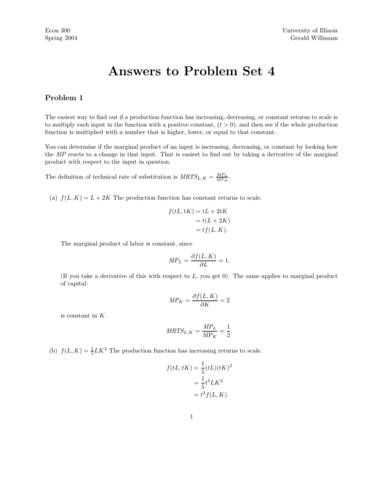
Econ 300
Spring 2004
University of Illinois
Gerald Willmann
Answers to Problem Set 4
Problem 1
The easiest way to find out if a production function has increasing, decreasing, or constant returns to scale is
to multiply each input in the function with a positive constant, (t > 0), and then see if the whole production
function is multiplied with a number that is higher, lower, or equal to that constant.
You can determine if the marginal product of an input is increasing, decreasing, or constant by looking how
the MP reacts to a change in that input. That is easiest to find out by taking a derivative of the marginal
product with respect to the input in question.
The definition of technical rate of substitution is MRTSL,K =
MPL
MPK .
(a) f (L, K) = L + 2K The production function has constant returns to scale.
f (tL, tK) = tL + 2tK
= t(L + 2K)
= tf (L, K).
The marginal product of labor is constant, since
∂f (L, K)
= 1.
∂L
MPL =
(If you take a derivative of this with respect to L, you get 0). The same applies to marginal product
of capital:
MPK =
∂f (L, K)
=2
∂K
is constant in K.
MRTSL,K =
MPL
1
= .
MPK
2
(b) f (L, K) = 15 LK 2 The production function has increasing returns to scale.
1
(tL)(tK)2
5
1
= t3 LK 2
5
= t3 f (L, K).
f (tL, tK) =
1
The marginal product of labor is constant
∂f (L, K)
∂L
K2
=
.
5
MPL =
The marginal product of capital is increasing
∂f (L, K)
∂K
2L
=
K and
5
2L
=
> 0.
5
MPK =
∂MPK
∂K
MRTSL,K =
1
K
MPL
=
.
MPK
2L
3
(c) f (L, K) = L 4 K 4 This function has constant returns to scale.
3
1
f (tL, tK) = (tL) 4 (tK) 4
1
3
= tL 4 K 4
= tf (L, K).
Marginal product of labor is diminishing.
1 −3 3
L 4 K 4 and
4
3
3
7
= − L− 4 K 4 < 0.
16
MPL =
∂MPL
∂L
Marginal product of capital is decreasing in K.
3 14 − 41
and
L K
4
5
3 1
= − L 4 K − 4 < 0.
16
MPK =
∂MPK
∂K
MRTSL,K =
3
1 − 34
K4
4L
3 14
− 41
4L K
=
K
.
3L
3
1
1
The production function has constant returns to scale.
(d) f (L, K) = L 3 + K 3
3
1
1
f (tL, tK) = (tL) 3 + (tK) 3
h 1 1
i3
1
= t3 L3 + K 3
3
1
1
= t L3 + K 3
= tf (L, K).
2
MPL decreases in L.
1
2
1
MPL = 3 L 3 + K 3
2
1
1
= L 3 + 2L 3 K 3
1
1
∂MPL
∂L
1 −2
L 3
3
2
2
+ K 3 L− 3
2
2
= 1 + 2L− 3 K 3 + L− 3 K 3 and
2
4
5
1
2
2
= − L− 3 K 3 − L− 3 K 3 < 0.
3
3
MPK decreases in K.
2
1
1
MPK = 3 L 3 + K 3
2
1
1
= L 3 + 2L 3 K 3
1
1
∂MPK
∂K
1 −2
K 3
3
2
2
+ K 3 K− 3
2
2
= 1 + 2L 3 K − 3 + L 3 K − 3 and
5
2 1
4
2 2
= − L 3 K − 3 − L 3 K − 3 < 0.
3
3
MRTSL,K
2
1
1
1 − 23
3 L3 + K 3
3L
= 2
1
1
1 − 32
3 L3 + K 3
3K
23
K
=
L
Problem 2
(a) The minimization problem
min wL + rK
s.t.
Q = ALα K β
can be written as a Lagrangean
Λ = wL + rK − λ(ALα K β − Q).
The first order conditions are:
∂Λ
= w − λαALα−1 K β = 0
∂L
∂Λ
= w − λβALα K β−1 = 0
∂K
∂Λ
= −ALα K β + Q = 0.
∂λ
We can modify the first equation to have
λ=
w
αALα−1 K β
3
Using this in the second equation gives
wβALα K β−1
wβL
=
α−1
β
αAL
K
αK
wL
rK
⇐⇒
=
.
α
β
r=
Since the MRTSL,K for this function only depends on the ratio of K to L, the expansion path is linear.
(Or more generally, the expansion path is linear for homothetic functions).
(b) With A = 2, α = β = 21 , and K = K̄, we have
1
1
Q = 2L 2 K̄ 2
Now
1
min wL + rK̄
1
s.t. Q = 2L 2 K̄ 2
Implies
1
L2 =
Q
2K̄
=⇒ L =
1
2
The short run cost function is
c(w, r, Q, K̄) = w
Q2
4K̄
Q2
+ rK̄.
4K̄
(c) To find the optimal amount of capital, we look at the firm’s cost minimization problem
1
min wL + rK
1
s.t. Q = 2L 2 K 2 ,
and build a Lagrangean
1
1
Λ = wL + rK − λ(2L 2 K 2 − Q).
From the first order conditions
1
1
∂Λ
= w − λL− 2 K 2 = 0,
∂L
1
1
∂Λ
= r − λL 2 K − 2 = 0, and
∂K
1
1
∂Λ
= −2L 2 K 2 + Q = 0
∂λ
we can solve λ (using the first equation) as
λ=
w
1
1
L− 2 K 2
.
Using this in the second equation gives us
1
r=
1
wL 2 K − 2
1
1
L− 2 K 2
=⇒ L =
=
wL
K
r
K.
w
Using this in the third equation gives us the optimal K:
r 21
r 12 1
K
Q=2
K K2 = 2
w
w
1 w 12
=⇒ K =
Q.
2 r
4
We can also see that the optimal amount of labor is
L=
r
1 r 12
Q.
K=
w
2 w
(d) The long run total cost function tells us the minimal costs needed to produce Q units of output:
c(w, r, Q) = wL(w, r, Q) + rK(w, r, Q)
1 r 12
1 w 12
=w
Q+r
Q
2 w
2 r
1
= (wr) 2 Q.
5
Question 3
a) Problem: Max (L, K): p L1/3 K 1/3 – wL – rK
FOC:
∂π / ∂L = p 1/3 L -2/3 K 1/3 = w
∂π / ∂K = p 1/3 L 1/3 K -2/3 = r
The first equation gives: L =
p3
27 w2 r
Plug into the second equation:
p
3
Then, L =
And K
1/ 3
p
1/ 3
L
p
9w
2
2
L
4/3
=r
3
27 w2 r
=
p3
3w(
)2 / 3
27 w2 r
p
1/ 3 w
1/ 3
so K =
p3
27 r 2 w
p
Finally, Q = L ( L) and Qa * =
r
2w
w
+ rQ 3/ 2 ( )1/ 2 = 2Q 3/ 2 ( wr )1/ 2
r
b) The problem is Max (Q, L, K): pQ – wL – rK s.t. Q = L1/3 K 1/3
Then, £ = pQ – wL – rK + λ (Q - L1/3 K 1/3)
FOC:
∂£ / ∂L = w - λ 1/3 L -2/3 K 1/3 = 0
∂£ / ∂K = r - λ 1/3 L 1/3 K -2/3 = 0
∂£ / ∂ λ = Q - L1/3 K 1/3 = 0
From 1 and 2: w/r = K/L
Then
w
r
w
r
w
r
Q = L1/ 3 ( L)1/ 3 and L* = Q 3/ 2 ( )1/ 2 and K * = Q3/ 2 ( )1/ 2
And the Cost function is:
C *(Q) = w(
Q2
25
c) The problem is Max (Q): pQ – C(Q)
FOC: ∂π / ∂Q = p – MC = 0
+4
Q2
25
)=
wQ 2
25
w
+ rQ 3/ 2 ( )1/ 2 = 2Q 3/ 2 ( wr )1/ 2
r
From C(Q): MC = 3 (wr)1/2 Q1/2
1/2
Then p = 3 (wr)
1/2
Q
and
Q* = (
p2
9 wr
)
Plug this Q* into the conditional factor demands of point b to get:
L* =
p3
27 w2 r
and K * =
p3
27 r 2 w
Question 4
a) Cost minimization
For firm A: Qa = La1/2 so La = Qa2 and C(La) = w Qa2
For firm B: Qb = 2 Lb1/2 so Lb = Qb2 / 4 and C(Lb) = w Qb2 / 4
Profit maximization:
For firm A: Max (Qa): p Qa – w Qa2
FOC:
∂π / ∂ Qa = p – 2 w Qa = 0 so Qa * =
p
2w
For firm B: Max (Qb): p Qb – w Qb2 / 4
FOC:
∂π / ∂ Qb = p – 2 w Qa = 0 so Qb * =
2p
w
b) Cost minimization for the joint firm:
Problem: Min (La, Lb): w (La + Lb) s.t. Q = La1/2 + 2 Lb1/2
Then, £ = w (La + Lb) = λ (Q - La1/2 + 2 Lb1/2 )
FOC :
∂£ / ∂La = w - λ 1/2 La -1/2 = 0
∂£ / ∂Lb = w - λ Lb -1/2 = 0
∂£ / ∂ λ = Q - La1/2 + 2 Lb1/2 = 0
Solving for w (1) and (2) and equalizing them:
1/2 La-1/2 = Lb-1/2 then 2 La1/2 = Lb1/2
Then Q = La1/2 + 2 Lb1/2 = La1/2 + 4 La1/2 = 5 La1/2
Solving this for La we get: La* = Q2 / 25 and then Lb* = 4 La = 4 Q2 / 25
Then C *(Q) = w(
Q2
25
+4
Q2
25
)=
wQ 2
5
Profit maximization for the joint firm:
Max (Q): p Q – C(Q)
FOC:
∂π / ∂ Q = p – MC = 0 and MC =
Q *=
2 wQ
5
so
5p
2w
c) Output supply
Is the function Q* = Q(p) that we found in point (b) so
Supply = Q * =
5p
2w
From cost minimization we found that:
2 La1/2 = Lb1/2 so 2 Qa = 1/2 Qb then 4Qa = Qb
Remember, MCa = 2w Qa
MCb = w/2 Qb = 2w Qa
So we see that marginal cost must be equal at both facilities.