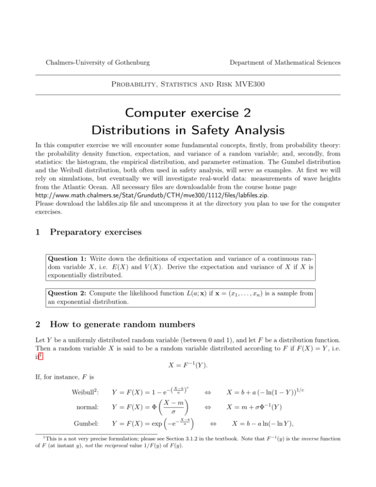
Chalmers-University of Gothenburg
Department of Mathematical Sciences
Probability, Statistics and Risk MVE300
Computer exercise 2
Distributions in Safety Analysis
In this computer exercise we will encounter some fundamental concepts, firstly, from probability theory:
the probability density function, expectation, and variance of a random variable; and, secondly, from
statistics: the histogram, the empirical distribution, and parameter estimation. The Gumbel distribution
and the Weibull distribution, both often used in safety analysis, will serve as examples. At first we will
rely on simulations, but eventually we will investigate real-world data: measurements of wave heights
from the Atlantic Ocean. All necessary files are downloadable from the course home page
http://www.math.chalmers.se/Stat/Grundutb/CTH/mve300/1112/files/labfiles.zip.
Please download the labfiles.zip file and uncompress it at the directory you plan to use for the computer
exercises.
1
Preparatory exercises
Question 1: Write down the definitions of expectation and variance of a continuous random variable X, i.e. E(X) and V (X). Derive the expectation and variance of X if X is
exponentially distributed.
Question 2: Compute the likelihood function L(a; x) if x = (x1 , . . . , xn ) is a sample from
an exponential distribution.
2
How to generate random numbers
Let Y be a uniformly distributed random variable (between 0 and 1), and let F be a distribution function.
Then a random variable X is said to be a random variable distributed according to F if F (X) = Y , i.e.
if1
X = F −1 (Y ).
If, for instance, F is
Weibull2 :
normal:
Gumbel:
X−b c
Y = F (X) = 1 − e−( a )
X −m
Y = F (X) = Φ
σ
X−b
Y = F (X) = exp −e− a
⇔
X = b + a (− ln(1 − Y ))1/c
⇔
X = m + σΦ−1 (Y )
⇔
X = b − a ln(− ln Y ),
This is a not very precise formulation; please see Section 3.1.2 in the textbook. Note that F −1 (y) is the inverse function
of F (at instant y), not the reciprocal value 1/F (y) of F (y).
1
Computer Exercise 2, MVE300
ii
then X is a Weibull, normally, and Gumbel distributed random variable, respectively. In Matlab uniformly random variables (“random numbers”) are generated by means of the command rand. We will use
it here to produce 500 Weibull-distributed random-numbers:
>> a=2; b=0; c=3.6;
>> x=b+a*(-log(1-rand(500,1))).^(1/c);
>> plot(x,’.’), grid on
Question 3: Why is there a full stop before the exponent on the second row in the Matlab
code here?
or 2000 normally-distributed random numbers:
>> m=10; sigma=3;
>> x=m+sigma*norminv(rand(2000,1));
>> plot(x,’.’), grid on
Here we really encourage you to use the command randn instead, i.e
>> x=m+sigma*randn(2000,1);
Eventually, produce 35 Gumbel-distributed random numbers:
>> a=2; b=3.6;
>> x=b-a*log(-log(rand(35,1)));
>> plot(x,’.’), grid on
Question 4: What do the plots look like? Do you see any regularity? Make any descriptive
comments on the type of data you see!
This type of plot may indicate the “average” value and spreading, but in the sequel we will illustrate
data graphically in a more convenient way. To generate random numbers in Matlab, one can also make
use of the commands wblrnd (Weibull), normrnd (normal), and raylrnd (Rayleigh) from the commercial
Statistics Toolbox.
3
Probability density function as a limit of histograms
In descriptive statistics the histogram is used as one way to describe the distribution of data. We will
now compare the histogram with the probability density function (pdf), often denoted by fX (x) if the
underlying random variable is X. In the following numerical example, X belongs to a Gumbel distribution
FX (x) = exp −e−(x−b)/a
with parameters a = 2, 1, b = 1, 7.
Generate 1000 observations:
>> a=2.1; b=1.7;
>> x=b-a*log(-log(rand(1,1000)));
2
Here, F is defined only for X > b, i.e when F (X) > 0
Computer Exercise 2, MVE300
iii
Question 5: Can you briefly explain what we did in the above lines of code?
To generate x, we can also make use of the Matlab Statistical Toolbox built-in command evrnd:
>> x=-evrnd(-b,a,1,1000);
The two minuses in the above command are needed because the Matlab uses the minimal value distribution
while the Gumbel distribution refers to the maximum value distribution (ambiguity of the word ’extreme’).
See Extreme Value Type I Distribution for more details. To avoid confusion, we have created Matlab
functions that allow to work with the Gumbel distribution with the same parametrization as in the
textbook. Now, we can run
>> x=gumbrnd(a,b,1,1000);
Next, make a histogram utilising the command hist:
>> help hist
>> hist(x)
Note that the number of observations in each class
R ∞is presented on the ordinata (y-axis). From theory, we
know that a pdf fX (x) always has the property −∞ fX (x) dx = 1. To compare the histogram with the
pdf, one has to scale the former.
Redraw the histogram using the bar function and rescaled height of the bars so the area of the bars
adds to one (this explains the presence of the term n/(sum(n)*(xout(2)-xout(1))) in the code below).
In the same figure, draw the theoretical pdf:
>>
>>
>>
>>
>>
>>
[n,xout]=hist(x);
bar(xout,n/(sum(n)*(xout(2)-xout(1))),1)
hold on
xv=linspace(min(x),max(x),1000);
plot(xv,exp(-(xv-b)/a-exp(-(xv-b)/a))/a,’r’)
hold off
Question 6: Do you understand what we have done here? Write down the probability
density function for X and identify it in the Matlab code above.
The Matlab routine evpdf gives the pdf for a Gumbel-distributed random variable, so it is also possible
to write (note that we used self-written gumbpdf rather than using Matlab’s evpdf which has the confusing
sign problem mentioned above):
>> [n,xout]=hist(x,100); % 100 in ’hist’ represents the number of bins for histogram
% you may change it to see what happens
>> bar(xout,n/(sum(n)*(xout(2)-xout(1)),1))
>> hold on
>> xv=linspace(min(x),max(x),500);
>> plot(xv,gumbpdf(xv,a,b),’r’)
>> hold off
Question 7: What would happen if you increased the number of generated values in xv?
(You may check by increasing 1000 to 2000 to 5000 to 10000.)
iv
Computer Exercise 2, MVE300
4
Expectation and variance of a random variable
For a random variable X, the expectation, sometimes called the mean and denoted E(X), gives the value of
X “on average”; if the distribution of X had been the mass distribution of a physical thing, the expectation
would have located
pthe centre of gravity of that thing. The variance V(X) (or, rather, the standard
deviation D(X) = V(X)) of X can be regarded as a measure of the distribution’s dispersion. For a set
of important distributions, E(X) and V(X) have been explicitely derived (in terms of the distribution’s
parameters) and tabulated, see for example the textbook.
For a given data set x1 , . . . , xn (sample), in most cases we do not know the distribution from which
the sample is taken,
and hence not the mean and variance of that distribution.
The sample mean, often
P
1 Pn
2
denoted x̄ = ( ni=1 xi )/n, and the sample variance, often denoted s2 = n−1
i=1 (xi − x̄) , are then the
corresponding measures of location and dispersion. If the number n of observations increases, we may
expect that these quantities become closer to E(X) and V(X) respectively. Let us examine this in Matlab
by means of simulated data, the distribution of which we can control:
Consider the Weibull distribution,
FX (x) = 1 − exp(−((x − b)/a)c ),
x ≥ b.
The mean and variance are given by
1
E(X) = b + a Γ(1 + ),
c
2
1 2
2
2
V(X) = a Γ(1 + ) − a Γ(1 + ) ,
c
c
where
Z
Γ(p) =
∞
xp−1 e−x dx.
(1)
0
is the gamma function. Choose for example a = 1, 5, b = 0, and c = 2. To calculate expectation and
variance, one needs the gamma function in (1) which is implemented in Matlab as gamma; hence
>>
>>
>>
>>
a=1.5; b=0; c=2;
EX=b+a*gamma(1+1/c)
VX=a^2*gamma(1+2/c)-a^2*(gamma(1+1/c))^2;
DX=sqrt(VX)
Now, simulate a sample of 50 observations and find the sample mean and standard deviation by the
commands mean and std respectively:
>> x=b+a*(-log(1-rand(1,50))).^(1/c);
>> mean(x), std(x)
(Again, can you understand this simulation?) Since b = 0, alternatively you can also use the Matlab
built-in routine wblrnd
>> x=wblrnd(a,c,1,50);
>> mean(x), std(x)
Question 8: Compare the values estimated from the samples with the theoretical values
EX, DX that you have also obtained above. Write down the values for E(X), x̄, D(X), d(x).
Are the theoretical and empirical values consistent with each other? Simulate larger samples
of, say, 200, 1000, and 5000 observations respectively. What happens when the number of
observations increases?
v
Computer Exercise 2, MVE300
5
Estimation of parameters
Assume that we have a sample x1 , . . . , xn from (for example) a Gumbel distribution, i.e. the distribution
function is
F (x) = exp −e−(x−b)/a .
However, the parameters a and b are not known. Then, one can use the maximum-likelihood method
(ML method) to estimate the parameters from the sample.
Question 9: Write down the likelihood function L(a, b; x) for the example above.
In the Statistical Toolbox the ML method has been implemented in evfit, wblfit, and raylfit for
the purpose of estimating the parameters in a Gumbel, Weibull, and Rayleigh distribution respectively.
First, simulate a sample of, say, 50 observations from a Gumbel distribution, then check if the
ML method implemented in gumbfit (which is based on evfit) returns good estimates:
>>
>>
>>
>>
>>
>>
a=2; b=3.5;
x=b-a*log(-log(rand(1,50)));
% Alternative 1
x=gumbrnd(a,b,1,50);
% Alternative 2
phat= gumbfit(x);
hata=phat(1)
hatb=phat(2)
Question 10: The parameter estimates are given in the vector phat. With the elements
phat(1) and phat(2) corresponding to b
a and bb, respectively. Compare the estimates b
a and
bb with the true values a and b! Write them down.
Properties of point estimates
The variances and covariances of the point estimates are always of interest. For the point estimates b
a and
bb of a and b in a Gumbel distribution above, the asymptotic variances and covariance (when the number
of observations “large”) are given by3
6 a2
a2
·
≈
0,
607
93
·
π2 n
2n
2
a2
a
6(1
−
γ)
V(bb) ≈
1+
≈
1,
108
67
·
·
π2
n
n
2
2
6(1 − γ) a
a
C(b
a, bb) ≈
·
≈ 0, 257 02 ·
π2
n
n
V(b
a) ≈
Question 11: Evaluate estimates of V(b
a), V(bb), and C(b
a, bb), using b
a instead of a, report
the obtained values.
3
def
It is not at all trivial to show this. Here, γ = limk→∞
P
k
i=1 (1/i)
− ln i = §0, 577 215 665 . . . is Euler’s constant (or
the Euler-Mascheroni constant to distinguish from e which is also frequently referred to as Euler’s constant); it is not known
whether γ is irrational or not (the seventh Hilbert problem)!
vi
Computer Exercise 2, MVE300
Estimation of quantiles
By means of b
a and bb, estimate the upper 1 % quantile, defined as the number x0,01 which satisfies
P(X > x0,01 ) = 0, 01 ⇔ 1 − F (x0,01 ) = 0, 01.
Thus, the equation
1 − exp −e−(x0,01 −b)/a = 0, 01
must be solved with respect to x0,01 ; we obtain
x0,01 = b − a ln(− ln(1 − 0, 01)).
A reasonable estimate x
[
0,01 of x0,01 would then be
b a ln(− ln(1 − 0, 01)).
x
[
0,01 = b − b
(2)
So it can be obtained from
>> xhat=phat(2)-phat(1)*log(-log(1-0.01))
Question 12: Get a numerical result (from the above) for the estimate of the quantile.
Since b
a and bb both are random variables, so is x
[
[
0,01 according to Equation (2). Then x
0,01 possesses an
expectation E([
x0,01 ) and a standard deviation D([
x0,01 ). The standard deviation indicates the dispersion
of the estimate x
[
,
and
it
is
therefore
important
to get an idea of the value of D([
x0,01 ). In most cases it
0,01
is impossible to find an exact value, and consequently an approximation has to do. Such an approximation
is called a standard error. By letting Z1 = bb, Z2 = b
a, c1 = 1, and c2 = − ln(− ln(1 − 0, 01)), we can make
use of the formula
V(c1 Z1 + c2 Z2 ) = c1 2 V(Z1 ) + c2 2 V(Z2 ) + 2c1 c2 C(Z1 , Z2 )
to obtain a standard error for x
[
0,01 :
r D([
x0.01 ) = V bb − b
a ln(− ln(1 − 0.01)) =
r
=
V(bb) +
2
− ln(− ln(0.99)) · V(b
a) + 2 · − ln(− ln(0.99)) · C(bb, b
a)
Question 13: Use approximations of V(b
a), V(bb), and C(bb, b
a) you got in Question 11 to
obtain the estimate of the standard deviation (aka standard error). Write down its numerical
value. Is it large comparing to the estimate value of quantile?
Of course, just 50 values to estimate x0,01 might be too small a number leading to a quite large
standard error.
Computer Exercise 2, MVE300
6
vii
Probability plots
Assume that we have a set of observations x1 , x2 , . . . , xn . Before we estimate any parameters, we must
convince ourselves that the observations originate from the right family of distributions, e.g. normal,
Gumbel, or Weibull. One way to get a rough idea of which family of distributions may be suitable, is to
display the observations in a probability plot 4 : If you suspect that the data originate from, for instance,
a normal distribution, then you should make a normal probability plot; if you instead suspect a Gumbel
distribution, then make a Gumbel probability plot. If, in the plot, the observations seem to line up well
along a straight line, it indicates that the chosen distribution for the probability plot indeed might serve
as a good model for the observations. Statistics Toolbox provides normplot (for normal distribution),
wblplot (for Weibull distribution); but unfortunately there is no probability plot for Gumbel distribution,
so we have created one and named it gumbplot (available in labfiles). Acquaint yourself with the abovementioned commands, for example
>>
>>
>>
>>
>>
>>
>>
>>
>>
>>
>>
dat1=randn(2000,1); % Attention: Normal distribution!
normplot(dat1)
wblplot(dat1)
dat2=rand(3000,1); % Attention: Uniform distribution!
normplot(dat2)
gumbplot(dat2)
dat3=wblrnd(2,2.3,1,3000); % Attention: Weibull distribution!
wblplot(dat3)
gumbplot(dat3)
% Attention: Gumbel distribution!
dat4=gumbrnd(1,2,1,3500);
% Available in labfiles
gumbplot(dat4)
Experiment more with the number of observations; change also distributions!
Question 14: What happens when you plot the data in the “wrong” distribution plot?
Measurements of significant wave heights in the Atlantic Ocean
In the field of oceanography and marine technology, statistical extreme-value theory has been used to a
great extent. In design of offshore structures knowledge about “extreme” conditions is important.
In the numerical examples above, we used artificial data, simulated from a distribution which we could
control. We will now consider real measurements from the Atlantic Ocean. The data set contains so-called
significant wave heights (in meters), that is, the average of the highest one-third of the waves.
Now, load the data set atlantic.dat and read about the measurements; then find the size of data,
and plot it:
>>
>>
>>
>>
atl=load(’atlantic.dat’);
help atlantic
size(atl)
plot(atl,’.’)
4
Before the computer age, the observations were plotted manually into diagram-forms printed on sheets of paper; therefore
we now and then will use the expression “to plot data in a certain probability paper” even if we are referring to computerdisplayed diagrams.
Computer Exercise 2, MVE300
viii
One knows that, roughly speaking, the registered so-called significant wave-heights behave, statistically,
as if they were maximum wave-heights; therefore one can suspect them to originate from a Gumbel
distribution, for instance. Below we will make different probability plots.
>>
>>
>>
>>
normplot(atl)
normplot(log(atl))
gumbplot(atl)
wblplot(atl)
Question 15: Which distribution might be a satisfactory choice? Estimate parameters as
in Section 5 for the distribution of your choice (gumbfit, wblfit, normfit).