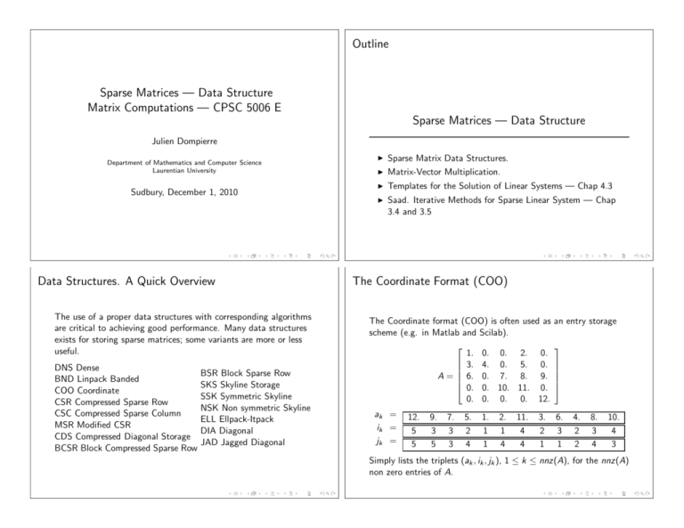
Outline
Sparse Matrices — Data Structure
Matrix Computations — CPSC 5006 E
Sparse Matrices — Data Structure
Julien Dompierre
Department of Mathematics and Computer Science
Laurentian University
Sudbury, December 1, 2010
Data Structures. A Quick Overview
The use of a proper data structures with corresponding algorithms
are critical to achieving good performance. Many data structures
exists for storing sparse matrices; some variants are more or less
useful.
DNS Dense
BND Linpack Banded
COO Coordinate
CSR Compressed Sparse Row
CSC Compressed Sparse Column
MSR Modified CSR
CDS Compressed Diagonal Storage
BCSR Block Compressed Sparse Row
BSR Block Sparse Row
SKS Skyline Storage
SSK Symmetric Skyline
NSK Non symmetric Skyline
ELL Ellpack-Itpack
DIA Diagonal
JAD Jagged Diagonal
◮
Sparse Matrix Data Structures.
◮
Matrix-Vector Multiplication.
◮
Templates for the Solution of Linear Systems — Chap 4.3
◮
Saad. Iterative Methods for Sparse Linear System — Chap
3.4 and 3.5
The Coordinate Format (COO)
The Coordinate format (COO) is often used as
scheme (e.g. in Matlab and Scilab).

1. 0. 0. 2. 0.
 3. 4. 0. 5. 0.

A=
 6. 0. 7. 8. 9.
 0. 0. 10. 11. 0.
0. 0. 0. 0. 12.
ak =
ik =
jk =
12.
5
5
9.
3
5
7.
3
3
5.
2
4
1.
1
1
2.
1
4
11.
4
4
3.
2
1
an entry storage






6.
3
1
4.
2
2
8.
3
4
10.
4
3
Simply lists the triplets (ak , ik , jk ), 1 ≤ k ≤ nnz(A), for the nnz(A)
non zero entries of A.
Matrix-Vector Product with the COO format
Matrix-Vector Product with the COO format
The sparse transpose matrix vector update y = AT x + y using
COO format is expressed
The sparse matrix vector update y = Ax + y using COO format is
expressed
yi k = yi k + a k xj k ,
1 ≤ k ≤ nnz(A).
yj k = yj k + a k xi k ,
Algorithm 1 COO sparse matrix vector update. The sparse
matrix A is given as nnz(A) triplets (ak , ik , jk ).
1: for k = 1 : nnz(A)
2:
y (ik ) = y (ik ) + a(k) ∗ x(jk )
3: end
Algorithm 2 COO sparse transpose matrix vector update. The
sparse matrix A is given as nnz(A) triplets (ak , ik , jk ). Then the non
zero elements of AT are given by the nnz(A) triplets (ak , jk , ik ).
1: for k = 1 : nnz(A)
2:
y (jk ) = y (jk ) + a(k) ∗ x(ik )
3: end
What is the complexity of this sparse matrix-vector multiplication
algorithm?
So, the sparse transpose matrix vector multiplication can be done
without explicitely creating the transpose matrix.
The Compressed Sparse Row (CSR) Format
Matrix Vector Product with the CSR Format
The Compressed Sparse Row (CSR) format is a common working
scheme.


1. 0. 0. 2. 0.
 3. 4. 0. 5. 0. 



A=
6.
0.
7.
8.
9.


 0. 0. 10. 11. 0. 
0. 0. 0. 0. 12.
ak
jk
ki
ki
=
=
=
=
1.
1
1
1
2.
4
3
3.
1
3
6
4.
2
5.
4
10
12
6.
1
6
13
7.
3
8.
4
9.
5
10.
3
10
1 ≤ k ≤ nnz(A).
11.
4
12.
5
12
Stores non zero entries ak row by row and their column index jk
are listed. Then, the index of the first entry k of each row i are
stored in ki . Also: Compressed Sparse Column (CSC) + variants
The sparse matrix vector update y = Ax + y using CSR format is
expressed
ki +1 −1
X
yi = yi +
a k xj k ,
1≤i ≤n
k=ki
13
Algorithm 3 CSR sparse matrix vector update. The sparse matrix A is given with the CSR format.
1: for i = 1 : n
2:
for k = ki : ki +1 − 1
3:
y (i ) = y (i ) + a(k) ∗ x(jk )
4:
end
5: end
Transpose Matrix Vector Product with the CSR Format
The Diagonal (DIA) Format

For the sparse transpose matrix vector update y = AT x + y using
CSR format, traversing columns of the matrix would be an
extremely inefficient operation.
Algorithm 4 CSR sparse transpose matrix vector update. The
sparse matrix A is given with the CSR format.
1: for i = 1 : n
2:
for k = ki : ki +1 − 1
3:
y (jk ) = y (jk ) + a(k) ∗ x(i )
4:
end
5: end
The Ellpack-Itpack Format
1. 0. 2. 0. 0.
 3. 4. 0. 5. 0.

A=
 0. 6. 7. 0. 8.
 0. 0. 9. 10. 0.
0. 0. 0. 11. 12.
AC =
2.
4.
7.
10.
12.
0.
5.
8.
0.
0.
DA =
⋆
3.
6.
9.
11.
1.
4.
7.
10.
12.
0.
4.
6.
0.
0.
2.
5.
8.
⋆
⋆
2. 0. 0.
0. 5. 0.
7. 0. 8.
9. 10. 0.
0. 11. 12.
IOFF =






-1
0
2
Block Matrices

1.
3.
6.
9.
11.


A=


1.
3.
0.
0.
0.
JC =
1
1
2
3
4





A=








3
2
3
4
5
1
4
5
4
5
AA =
1.
5.
2.
6.
3.
7.
4.
8.
JA =
1
5
1. 2. 0. 0. 3. 4.
5. 6. 0. 0. 7. 8.
0. 0. 9. 10. 11. 12.
0. 0. 13. 14. 15. 16.
17. 18. 0. 0. 20. 21.
22. 23. 0. 0. 24. 25.
9.
13.
10.
14.
3
5
11.
15.
12.
16.
1
17.
22.
18.
23.
5








20.
24.
21.
25.
IA =
1
3
5
Each column in AA holds a 2 × 2 block. JA(k)= col. index of
(1,1) entries of the k-th block.
7
Why So Many Sparse Data Structure?
The Dompierre’s Law
In 1975, Niklaus Wirth wrote the book “Algorithms + Data
Structures = Programs”.
Performance can vary significantly for the same operation.
Storage Scheme / Kernel
Compressed Sparse Row
Compressed Sparse Column
Ellpack-Itpack
Diagonal
Diagonal Unrolled
CRAY-2
8.5
14.5
31
66.5
99
Alliant
7.96
0.6
6.72
9.53
13.92
MFLPS for matrix-vector ope s on CRAY-2 and Alliant FX-8 [From
sparse matrix benchmark, (Wijshoff and Saad, 1989)]
Best algorithm for one machine may be worst for another.
Theorem (Dompierre’s Law)
Algorithms + Data Structures + Computer Architecture =
Programs