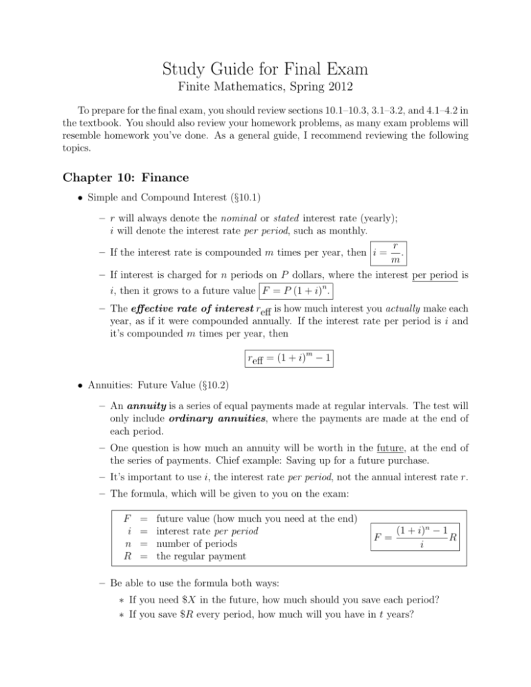
Study Guide for Final Exam
Finite Mathematics, Spring 2012
To prepare for the final exam, you should review sections 10.1–10.3, 3.1–3.2, and 4.1–4.2 in
the textbook. You should also review your homework problems, as many exam problems will
resemble homework you’ve done. As a general guide, I recommend reviewing the following
topics.
Chapter 10: Finance
• Simple and Compound Interest (§10.1)
– r will always denote the nominal or stated interest rate (yearly);
i will denote the interest rate per period, such as monthly.
r
– If the interest rate is compounded m times per year, then i = .
m
– If interest is charged for n periods on P dollars, where the interest per period is
i, then it grows to a future value F = P (1 + i)n .
– The effective rate of interest reff is how much interest you actually make each
year, as if it were compounded annually. If the interest rate per period is i and
it’s compounded m times per year, then
reff = (1 + i)m − 1
• Annuities: Future Value (§10.2)
– An annuity is a series of equal payments made at regular intervals. The test will
only include ordinary annuities, where the payments are made at the end of
each period.
– One question is how much an annuity will be worth in the future, at the end of
the series of payments. Chief example: Saving up for a future purchase.
– It’s important to use i, the interest rate per period, not the annual interest rate r.
– The formula, which will be given to you on the exam:
F
i
n
R
=
=
=
=
future value (how much you need at the end)
interest rate per period
number of periods
the regular payment
F =
(1 + i)n − 1
R
i
– Be able to use the formula both ways:
∗ If you need $X in the future, how much should you save each period?
∗ If you save $R every period, how much will you have in t years?
Final Exam Study Guide
Page 2 of 3
Finite Math, Spring 2012
• Annuities: Present Value (§§10.2–10.3)
– Another question is how much an annuity of payments stretching into the future
is worth now.
– The most important example: the amount of money the bank loans you now is
worth a series of loan payments you’ll make to them over the next several years.
– Another example: you have a lump of money in the bank now from which you
will make regular payments over the next few years.
– The formula, which will be given to you on the exam:
P
i
n
R
=
=
=
=
present value (how much you need now)
interest rate per period
number of periods
the regular payment
P =
1 − (1 + i)−n
R
i
– Be able to use the formula both ways:
∗ If you take out a loan of $X now, how much will the regular payments be?
∗ If you can afford monthly payments of $R, how much of a loan can you take
out now?
Chapter 3: Linear Programming
• Linear Programming: Graphing Feasible Regions
– Given a description of the problem in words, convert it to a system of inequalities and the objective function.
1. What do you get to control? What decisions do you make? Those will be
your variables.
2. Make a chart of the information presented, looking roughly like this:
choice 1 choice 2 Available
resource 1
resource 2
..
.
3. Convert each row of the chart into an inequality.
4. Be ready in case some inequalities are expressed in other terms (e.g. “you
must have twice as many widgets as sprockets”)!
5. Don’t forget the reality constraints, which usually look like x ≥ 0.
– Given a system of inequalities, graph the feasible region.
1. For each inequality, graph the corresponding equality as a line.
2. Next, for each inequality, determine which side of the line is “good,” and
cross out the “bad” side by shading it.
3. The feasible region is the remaining white space.
Final Exam Study Guide
Page 3 of 3
Finite Math, Spring 2012
– Find the coordinates of each corner of the feasible region. (You can probably
solve these without Gauss-Jordan, just by substitution or adding & subtracting.)
• Linear Programming: Optimization
– Given a linear programming problem, solve it as follows:
1. Interpret the problem to get the system of inequalities and the objective
function.
2. Graph the feasible region.
3. Find and label all corner points.
4. Evaluate the objective function at each corner point.
5. If the maximum occurs at just one corner, that is the only place where it
occurs.
6. If the maximum occurs at two corners, then it occurs along the whole edge
joining them.
Chapter 4: The Simplex Method
• Be able to convert a linear programming problem into a tableau.
• Be able to read a tableau and understand what it means in terms of equations and
inequalities.
• Be able to read off the “silly solution” represented by a tableau.
1. Recognize which variables are “pretty” (all zero columns, except for a single 1)
and which are “ugly.”
2. Plug in zero for the ugly variables.
3. Solve for the pretty variables.
• Be able to pivot a tableau around a designated entry.
1. If the entry has value k, divide its entire row by k to change the entry to 1.
2. Now add multiples of that row to the other rows to make the rest of that column
zero.
• Be able to decide which entry to pivot around:
1. Find the entry in the last row that is the most negative. Pivot in that column.
2. For each row, divide the last column’s entry by the entry in the pivot column to
get a quotient. Choose to pivot in the row with the smallest nonnegative quotient.
• Recognize when a tableau represents the maximal solution.
– (All entries in the last row are positive.)