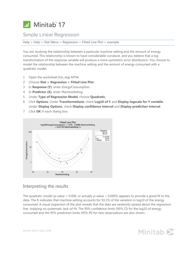
Simple Linear Regression
Help > Help > Stat Menu > Regression > Fitted Line Plot > example
You are studying the relationship between a particular machine setting and the amount of energy
consumed. This relationship is known to have considerable curvature, and you believe that a log
transformation of the response variable will produce a more symmetric error distribution. You choose to
model the relationship between the machine setting and the amount of energy consumed with a
quadratic model.
1
Open the worksheet Exh_regr.MTW.
2
Choose Stat > Regression > Fitted Line Plot.
3
In Response (Y), enter EnergyConsumption.
4
In Predictor (X), enter MachineSetting.
5
Under Type of Regression Model, choose Quadratic.
6
Click Options. Under Transformations, check Log10 of Y and Display logscale for Y variable.
Under Display Options, check Display confidence interval and Display prediction interval.
7
Click OK in each dialog box.
Interpreting the results
The quadratic model (p-value = 0.000, or actually p-value < 0.0005) appears to provide a good fit to the
data. The R indicates that machine setting accounts for 93.1% of the variation in log10 of the energy
consumed. A visual inspection of the plot reveals that the data are randomly spread about the regression
line, implying no systematic lack-of-fit. The 95% confidence limits (95% CI) for the log10 of energy
consumed and the 95% prediction limits (95% PI) for new observations are also shown.
WWW.MINITAB.COM