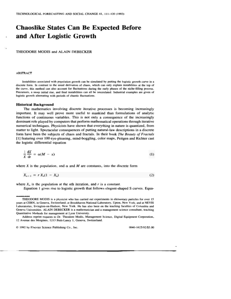
TECHNOLOGICAL FORECASTING AND SOCIAL CHANGE 41, 111-120 (1992)
-
Chaoslike States Can Be Expected Before
and After Logistic Growth
THEODORE MODIS and ALAIN DEBECKER
ABSTRACT
Instabilities associated with population growth can be simulated by putting the logistic growth curve in a
discrete form. In contrast to the usual derivation of chaos, which can only explain instabilities at the top of
the curve, this method can also account for fluctuations during the early phases of the niche-filling process.
Precursors, a steep initial rise, and final instabilities can all be interrelated. Industrial examples are given of
logistic growth alternating with periods of chaotic fluctuations.
Historical Background
The mathematics involving discrete iterative processes is becoming increasingly
important. It may well prove more useful to mankind than formulations of analytic
functions of continuous variables. This is not only a consequence of the increasingly
dominant role played by computers that perform mathematical operations through iterative
numerical techniques. Physicists have shown that everything in nature is quantized, from
matter to light. Spectacular consequences of putting natural-law descriptions in a discrete
form have been the subjects of chaos and fractals. In their book The Beauty ofFructuls
[ 11 featuring over 100 eye-pleasing, mind-boggling, color maps, Peitgen and Richter cast
the logistic differential equation
_1 d_X
X dt
= a ( M - x)
where X is the population, and a and M are constants, into the discrete form
where X,, is the population at the nth iteration, and r is a constant.
Equation I gives rise to logistic growth that follows elegant-shaped S curves. EquaTHEODORE MODIS is a physicist who has carried out experiments in elementary particles for over 15
years at CERN, in Geneva, Switzerland; at Brookhaven National Laboratory, Upton, New York; and at NEWS
Laboratories, Irvington-on-Hudson, New York. He has also been on the teaching faculties of Columbia and
Geneva Universities. ALAIN DEBECKER is a mathematician and a management science consultant, teaching
Quantitative Methods for management at Lyon University.
Address reprint requests to Dr. Theodore Modis, Management Science, Digital Equipment Corporation,
12 Avenue des Morgines, 1213 Petit-Lancy 1, Geneva, Switzerland.
0 1992 by Elsevier Science Publishing Co., Inc.
0040-1625/92/$5.00
T. MODIS AND A. DEBECKER
112
tion 2 leads to states of chaos and the fascinating world of fractals. The bridge between
continuous and discrete formulations spans 150 years of developments in mathematics.
It starts with Verhulst [2] finishes with Mandelbrot [3] and intricately links order with
chaos.
The work reported here also links logistic growth to erratic fluctuations, but through
a somewhat different approach. Our motivation was not to study chaos. We were simply
trying to find ways to speed up a computer program. Working for a computer company,
one is often spoilt because there are usually unlimited computing resources. Nevertheless,
human nature is such that having does not quench greed. When we realized that it required
more than a few minutes of real-time computing, for the minimization of a x2 involving
the convolution of two logistic functions, we found the situation unacceptable [4]. Instead
of searching for a programming trick that would accelerate the process, we used a
mathematical trick. In constructing the S curve, we replaced the analytic function by an
iterative process. We obtained the familiar logistic-growth pattern, but, in addition, we
observed chaoslike states before and after the steep rise.
This finding came as an ex machina deus because important fluctuations at the
extremities of S curves had often been observed and had served as ammunition to critics
of logistic-growth applications.
Making an S Curve Discrete
Maede [5] has shown that logistic growth can be obtained through a simple hyperbola
in the recursive relation:
where a and b are constants and there is a third constant involved, the starting value Xo.
Such iterative operations produce S curves like the solutions of equation 1. This approach
is different from the one of chaos scientists who first put the differential equation in a
discrete form--equation 2-and then iterate it. We essentially put the solurion of the
differential equation in a discrete form.
A mathematically equivalent form of equation 3 is the following:
where M is the niche size just as in equation 1, and k can be linked to the constant a of
equation 1 through such a relationship as k = ed. Equation 4 leads to
xrl
--
M
-
X,
- u k”
where u
=
XO
M - Xo
We see that, with time (that is, as n increases), this quantity converges toward 0 or
00, depending on Ikl. IF IkI > 1, the population X , grows toward M , which behaves
as an attractor. For Ikl < 1, the population decreases toward 0, which now becomes the
attractor, while M behaves like a repeller. The relationship between successive terms X ,
can be seen pictorially in Figure la. The population curve traces out the familiar S shape
of logistic growth.
+
.
113
CHAOSLIKE STATES AND LOGISTIC GROWTH
a
'n+l
x1
x3
M
x2
/
b
I
I
I
I
I
I
I
x1
x"
Fig. 1. Iterations of a hyperbola. Graphs of equation 4 (the thin line indicates the sequence of terms):
(a) k > 1, a monotonic approach to the value M ; and (b) k < 0 , convergence following excursions above
and below M .
T. MODIS AND A. DEBECKER
114
For equation 4,it is natural that k > 0. However, in equation 3, proposed by Maede
and used in our iteration, the sign of k-a nontrivial formulation in terms of a and &
was not something we thought constraining. So we observed the consequences of having
k < 0, namely, oscillations. Successive terms of the sequence X n oscillate around the
end value M ,as indicated in Figure lb. The population goes through an overshoot, falls
back, and proceeds through oscillations of diminishing amplitude after which it stabilizes
at the value M.
Negative values for the constant k imply complex values for the constant a of the
logistic equation 1. The modulus of k is related to the steepness of the growth while its
argument determines the frequency of the oscillations. Complex values for ci and k
produced the states shown in Figure 2. At the top, we see the beginning of an oscillation.
For some values of the parameters, we obtain the rapid oscillations shown in Figure 2b.
At the bottom, we see a case with an irrational period yielding irregular fluctuations. In
all cases, the oscillations precede as well as follow the logistic growth.
The states of Figure 2 resemble publicized pictures obtained by chaos scientists via
equation 2 [6]. Our approach, however, does not lead to true chaos. The oscillations we
observe die out sooner or later; the damping constant can be large, but is not infinite.
We have used the hyperbolic function, equation 3, instead of the parabolic one, equation
2. Consequently, our series is a reversible one; from late values, one can reconstruct
early ones, which is not the case with true chaos. We can also interpolate the discrete
points indefinitely thus recovering a smooth curve, which again is not possible with chaos.
The smooth curve that can be recovered from formula 5 is the solution of equation 1,
namely, the familiar logistic growth:
but with a complex, to is a simple constant.
Upon approaching the ceiling, the discrete form-Figure 2c-shows erratic instabilities not unlike those observed in chaotic states, but with an additional new feature.
Instabilities are now also encountered before the main thrust of the growth.
For true chaos obtained via equation 2, the amount of irregularity is linked to the
magnitude of r. As r increases, one witnesses the onset of oscillations first simple, then
complicated, and eventually chaos. In our approach, it is the arg(k) that gives rise to the
oscillations, while Ikl only relates to the steepness of the growth and the damping constant
of the oscillations. The dependence on k is as follows:
0
0
0
0
For arg(k) = 0, that is, a real, we obtain the classic logistic growth.
For arg(k) = T , that is, k < 0, we observe regular oscillations alternating above
and below M.
For arg(k) = ( p / q ) 2 ~ where
,
p and q are prime integers, the series oscillates
with period q.
Finally, when arg(k) is an irrational multiple of T , then there is nonrepeating
fluctuations resembling true chaos patterns.
Rather than upon crossing a threshold value (as for the parameter r ) , our chaos
appears for a dense subset of the parameter k impacting the oscillation period.
-
CHAOSLIKE STATES AND LOGISTIC GROWTH
115
$
I
1
\
1
*.
I
a
b
C
Fig. 2. Making an S curve discrete. These are examples of the patterns obtained by varying the
parameters in the discrete formulation of the logistic growth function. (a) The so-called catching-up effect
and the possibility of precursor and overshoot. The line appears smooth because of rapid sampling. (b)
Regular oscillations. (c) States resembling chaos. In all cases, similar behavior is observed before as well
as after the main growth phase.
T. MODIS AND A. DEBECKER
116
Annual registrations
in millions
3
2
1
0
1950
a
1960
1970
1980
Billions of
of square feet
20
16
12
8
4
-
n
b
1940
1950
1960
Year
1970
1980
Fig. 3. (a) This graph shows data for
new car registrations in Japan as reported by Marchetti [8]. (b) This graph
is taken from the article of Montrey
and Utterback [9] and shows the annual plywood sales in the United States.
In both cases, significantdeviationsfrom
a logistic pattern appear when the ceiling is approached.
Deviations at Both Extremities of the S Curve
When chaos studies first diffused through the media, they were welcomed by logisticgrowth advocates who were in need of an explanation for the anomalies they had encountered. The annual rate of a population growth into a new niche had often been seen
to follow a logistic pattern that brakes into fluctuations of random character and sizable
amplitude just before reaching the ceiling.' Two such examples are shown in Figure 3,
the number of new car registrations in Japan as reported by Marchetti, and the annual
sales of plywood in the United States as reported by Montrey and Utterback.[9]. Both
processes follow a logistic-growth pattern developing significant random fluctuations as
the ceiling is approached. Chaos provides a mechanism for explaining these fluctuations.
'Such oscillations have been reported by Elliott Montroll and Wade Badger [7], and later by Cesare
Marchetti [S].
CHAOSLIKE STATES AND LOGISTIC GROWTH
117
Billions of tons
1000
tt
d
P
800
600
400
200
0
1850
1900
1950
2000
2050
Fig. 4. Annual production of bituminous coal in the United States [lo, 111. The S curves shown are
logistic fits to the data for the respective historical periods. The Interim period shows large fluctuations
of chaotic nature.
However, there have also been systematic deviations from logistic patterns during the
early phases of the growth. These deviations can not be explained by the classic chaos
formulation.
Marchetti in his numerous applications of logistic growth has characterized early
deviations from S curves in behavioral terms using such metaphors as “infant mortality”
and “catching-up effect.” With the former, he refers to unsuccessful competitive growth
before it reaches 10% of the ceiling. This phase can be considered as a trial period, during
which survival is at stake and major readjustments may be undertaken. Many young
organisms, not properly cared for, die during this period. By analogy, industrial products
are often repositioned pricewise and/or performancewise shortly after launching.
Marchetti’s second characterization refers to the sudden release of pent-up energy
following a “technical” delay in the early evolution of a population. It is manifested as
growth at an accelerated rate until the logistic trajectory is reached. Again, there is an
industrial analogue, a surge in sales with some product introductions.
The fluctuations preceding the logistic rise in Figure 2 provide an explanation for
the early irregularities mentioned above. In Figure 2a, we see the beginning of an oscillation before the S curve develops. Negative excursions of a population have no physical
meaning, so what is observed from the perturbation is a precursor and a steep rise toward
the logistic path. Marchetti would have said infant mortality followed by a catching-up
effect.
Variations in the annual rate of a population can be large, but they do not always
imply that we are simply witnessing the chaotic behavior that follows the completion of
a niche. The random fluctuations could equally well belong to a new growth process that
will fill up a new “market” niche. Such is the case depicted in Figure 4, of bituminous
coal production in the United States.* The large oscillations in the annual production of
coal between the years 1920 and 1960 may be seen as belonging to the ceiling of the
first S curve as well as to the beginning of the second one. In fact, had we had no
’Annual data for coal production come from the US Bureau of the Census [lo, 111.
T. MODIS AND A. DEBECKER
118
Percentage of total
60 --
50 -40 -30 -20 --
lot
I
I
I
I
I
historical data before 1950, we would have observed a deviation between data and curve
around 1960 that we would have rightfully interpreted as a catching-up effect.
As can be surmised from Figure 2a, the presence of a precursor should correlate
with a steeper initial rise, which in turn leads into an overshoot upon approaching the
ceiling. Such a picture is partially depicted by the data on oil imports in the United States
shown in Figure 5.3 Before 1969, there was a law limiting the amount of oil imported
in the United States to a fixed fraction of the total oil consumption. This shows up in
Figure 5 as a flat percentage until 1969. The fact, however, that the quota was consistently
met indicates a certain pressure on the constraining law. It was perhaps in response to
this pressure that the restriction was lifted in 1970. What followed is a sharp rise in the
percentage of imported oil reaching more than 60% ten years later, falling back to almost
30% in 1984 and rising significantly afterward. The logistic-growthcurve drawn in Figure
5 is an artistic interpretation of what a “natural” niche-filling process would have looked
like. The large-size oscillations around the 50% level might have been triggered by the
sharp rise of the early 1970s, itself a reaction to the long-term quota imposition.
The generalized picture is one of alternating states of logistic growth and chaos. A
clear example is the per capital energy consumption worldwide. Ausubel and colleagues,
sufficiently aware of this alternation, have built it into their forecasts. Figure 6, which
has been taken from their publication [ 131, shows three cycles of logistic growth followed
by chaos: two depicted by data and one forecasted by the authors.
Conclusions
Chaos studies, as they have been carried out so far, focus on what happens after
the niche is filled. The initial S-shaped rise is largely ignored by chaos scientists, who
are only interested in phenomena with erratic fluctuations. Many real cases, however,
like the production of coal and the world energy consumption shown earlier, display
multiple periods of growth. New markets open new niches and the historical picture
’An early version of Figure 5 can be found in Marchetti [12]
CHAOSLIKE STATES AND LOGISTIC GROWTH
119
/-
I
/
i
I
I
3
1
1
0
I
t
1
I
I
I
I
I
I
11
I
I
Futura
/
I
/'
2.17
I
I
I
I
I
I
I
f l ! ( I : 1 1
1
1850
I
0
I
I
Past
I
2
I
I
I
1900
1950
I
I l ! I I f I f
2000
2050
I
2100
Fig. 6. The per capita annual energy consumption worldwide. The graph published by Ausubel at
el. [13] shows data, logistic fits, and scenarios for the future.
becomes an alternation of logistic growth with periods of instability. The chaotic fluctuations belong to the end of a growth phase as much as to the beginning of the next
one. Associating a peak with the past as an overshoot, or with the future as a precursor,
is in some cases a simple question of taste.
The method described here for casting an S curve into a discrete form accounts for
instabilities at both ends of logistic growth. One could reasonably expect that an upcoming
growth phase in a new market niche will be heralded by precursors and, once installed,
will proceed at an accelerated rhythm in the beginning. Moreover, exploring the mathematical formulation (through variation of the parameters) can teach us how the frequency
and the importance of the precursors relate to the steepness and the size of the catching
up, which in turn affects the instabilities expected at the top.
There is one final remark. A well-established S curve will point to the time when
chaotic oscillations should be expected; it is when the ceiling is being approached. In
contrast, an entrenched chaos will reveal nothing about when the next growth phase will
start. One has to locate the next growth phase from other considerations particular to
each case. As suggested in the work of Ausubel et al. [13], the Kondratieff cycle is one
way to position growth periods. In both examples shown earlier, namely, coal production
in the United States and world energy consumption, there is coincidence between periods
of steep rise in growth and a Kondratieff upswing, namely, 1884-1912 and 1940-1968.
120
T. MODIS AND A. DEBECKER
References
1. Peitgen, H. O., and Richter, P. H.,The Beauty of Fractals, Springer-Verlag, Berlin, 1986.
2. Verhulst, P. F., Rechercher Mathdmatiques sur la h i d'Accroissement de la Population, in Nouveaux
Mimoires de I'Acadcfmie Royale des Sciences, et Belles-Lettres de Bruxelles, tome XVIII, 1 4 0 (1845).
3. Mandelbrot, B., The Fractal Geometry of Nature, Freeman, New York, 1977.
4. Modis, T., and Debecker, A., Determining the Services Life Cycle of Computers, in The Diffusion of
Technologies and Social Behavior, N. NakiCenoviC and A. Griibler, Springer-Verlag, Berlin, 1991.
5. Meade, N., Forecasting Using Growth Curves: An Adaptive Approach, Journal of the OperationalResearch
Society, 36(12), 1985, pp 1103-1115.
6. Gleick, J . , Chaos, Viking, New York, 1987, pp. 63-72.
7. Montroll, E. W., and Badger, W. W., Introduction to Quantitative Aspects of Social Phenomena, Gordon
and Breach, New York, 1974.
8. Marchetti, C., The Automobile in a System Context: The Past 80 Years and the Next 20 Years, Technological Forecasting and Social Change, 23, 3-23 (1983).
9. Montrey, H., and Utterback, J., Current Status and Future of Structural Panels in the Wood Products
Industry, Technological Forecasting and Social Change 38, 15-35, 1990.
10. Bureau of the Census, Statistical Abstract of the USA, Washington, DC, U . S . Government Printing Office,
1985- 1990.
11. Bureau of the Census, Historical Statistics of the United States, Colonial Times to 1970, Washington, DC,
U.S. Government Printing Office, 1975.
12. Marchetti, C., Energy Systems: The Broader Context, Technological Forecasting and Social Change 14,
191-203, 1979.
13. Ausubel, J., Griibler, A., and NakiCenoviC, N., Carbon Dioxide Emissions in a Methane Economy, Climatic
Change 12, 245-263, 1988.
Received 3 May 1991; revised 26 August 1991.