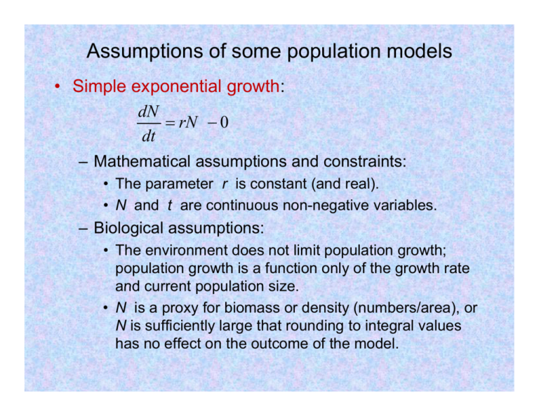
Assumptions of some population models
• Simple exponential growth:
dN
 rN  0
dt
– Mathematical assumptions and constraints:
• The parameter r is constant (and real)
real).
• N and t are continuous non-negative variables.
– Biological
g
assumptions:
p
• The environment does not limit population growth;
population growth is a function only of the growth rate
and current population size.
size
• N is a proxy for biomass or density (numbers/area), or
N is sufficiently large that rounding to integral values
h no effect
has
ff t on the
th outcome
t
off the
th model.
d l
Assumptions of some population models
• Monomolecular growth for reactant and product
(resources and population size):
R t   C t   A
dR
 0  kR,
d
dt
dC
 kR  0
ddt
– Mathematical assumptions and constraints:
• Parameters A and k are constant and non-negative.
non negative.
• R, C, and t are continuous non-negative variables.
– Biological assumptions:
• The environment (A) is absolutely limiting.
• R and C are proxies for concentrations of substances.
– E.g.,
E g resources and biomass
biomass.
• One unit of R is converted to one unit of C.
Assumptions of some population models
• Logistic growth:
 rN 2 
dN
 N
 rN 1    rN  

dt
 K
 K 
– Mathematical assumptions and constraints:
• Parameters r and K are constant; K is positive.
variables.
• N and t are continuous non-negative variables
– Biological assumptions:
• The environment (K) is absolutely limiting.
• N is a proxy for biomass or density (numbers/area), or
N is sufficiently large that rounding to integral values has
no effect on the outcome of the model.
Birth and death processes
• Population models in terms of birth and death:
B = instantaneous birth rate (number of births/time)
D = instantaneous death rate (number of deaths/time)
• Unlimited (exponential) population growth:
– Population growth rate r is just the difference
between constant birth rate and constant death rate
rate.
dN
 BN  DN
dt
  B  D N
 rN
Birth and death processes
• Li
Limited
it d (d
(density-dependent)
it d
d t) population
l ti growth:
th
dN
 BN  N  DN  N
dt
BN  f B  N  , DN  f D  N 
• For logistic growth:
• Functions fB and
fD are linear.
B0
DN  D0  dN
b
D0
r0  B0  D0
B0  D0
K
bd
d
BN  B0  bN
• Many other kinds
of functions are
possible.
Logistic model with time delay
• Logistic model: instantaneous growth rate at a given
instant is a function of the population size at that instant.
• Implies that factors that limit population growth are
assumed to act instantaneously on changes in
populations size, with no time delay.
• Realistically, there will be some delay (lag) before the
effects of a factor due to changing population size are
incorporated into the dynamics of the population
population.
• E.g., herbivore population may attain high numbers by
overgrazing a pasture.
– Will then decline due to food shortage until vegetation
recovers from effects of overgrazing.
• Time delay (lag) in response to limiting factors may lead
to fluctuations in population size.
Logistic model with time delay
• Modify logistic model to include lag:
– Let growth rate (and population size) at time t depend
on population size at time (t-tlag).
– Gives a delay-differential equation for rate of change
of population size:
 N  t  tlag  
dN  t 
 rN  t  1 

d
dt
K


– Can’t be solved (integrated) analytically.
– Can use numerical integration methods.
Logistic model with time delay
• Ex:
E th
three series
i corresponding
di tto:
r = 0.3, 1.2, 2.0
N0 = 2
2, K = 10
tlag = 1
• For increasing
g r,, population
p p
trajectory
j
y changes:
g
– r = 0.3: Steady increase to equilibrium K.
– r = 1.2: Damped oscillations converging on K.
– r = 2.0: Sustained oscillations (limit cycle).
Logistic model with time delay
• Fluctuations in population size due to lag:
– Occur because population can overshoot and fall below
q
before change
g in g
growth rate stems the
equilibrium
increase or decreases the decline.
– Dynamic behavior of model depends on relative
magnitudes
it d of:
f
• Intrinsic rate of increase, r.
• Time delay, tlag .
– Interaction modeled by the product r  tlag .
1
• 0  rtlag  e 
•
•
e 1  rtlag   2 
 2  rtlag

l 
:steady increase or decrease to
equilibrium.
:damped oscillations to equilibrium.
:limit cycles with amplitude and
frequency depending on rtlag .
Logistic model with time delay
• Behavior of model can be expressed in terms of
characteristic return time:
1
Tr 
r
= time taken to increase population size by a factor of
e = 2.718…,
2 718
growing exponentially with rate constant r.
r
– If time lag is long relative to characteristic return time:
• Population tends to overshoot and undershoot.
• Leads to cyclical fluctuations.
• Models with time lags can mimic fluctuations in natural
populations (voles, red grouse, lynx).
– Underlying biological mechanisms not well understood.
Generalization of the logistic model
• Logistic model assumes that birth and death rates
change linearly with increasing population size.
B0
DN  D0  dN
b
D0
d
BN  B0  bN
– Mathematical simplification (“model of ignorance”)
– No biological rationale for this assumption
assumption.
– Several generalizations have been proposed.
Generalizations of the logistic model
Birth rate
Pop
pulation size N
dN
 N
 rN 1  
• 2-parameter logistic model:
dt
 K
1


• 3-parameter generalization: dN  rN 1   N 
  K 
dt

   N  0    
 1
 r t
 

e
• Solution: N  t   K 1  1  

   K  





Population size N
Time




Generalizations of the logistic model
• Oth
Other generalizations
li ti
allow
ll
ffor more complicated
li t d
cases:
Birth rate
Birth rate
–E
E.g.,
g Allee effect: finding mates is more difficult when
population density is low.
Population size N
Population size N