NCSS Statistical Software
NCSS.com
Chapter 435
Multidimensional
Scaling
Introduction
Multidimensional scaling (MDS) is a technique that creates a map displaying the relative positions of a number of
objects, given only a table of the distances between them. The map may consist of one, two, three, or even more
dimensions. The program calculates either the metric or the non-metric solution. The table of distances is known as
the proximity matrix. It arises either directly from experiments or indirectly as a correlation matrix.
To understand how the proximity matrix may be observed directly, consider the following marketing research
example. Suppose ten subjects rate the similarities of six automobiles. That is, each subject rates the similarity of each
of the fifteen possible pairs. The ratings are on a scale from 1 to 10, with “1” meaning that the cars are identical in
every way and “10” meaning that the cars are as different as possible. The ratings are averaged across subjects,
forming a similarity matrix. MDS provides the marketing researcher with a map (scatter plot) of the six cars that
summarizes the results visually. This map shows the perceived differences between the cars.
The program offers two general methods for solving the MDS problem. The first is called Metric, or Classical,
Multidimensional Scaling (CMDS) because it tries to reproduce the original metric or distances. The second method,
called Non-Metric Multidimensional Scaling (NMMDS), assumes that only the ranks of the distances are known.
Hence, this method produces a map which tries to reproduce these ranks. The distances themselves are not
reproduced.
Discussion
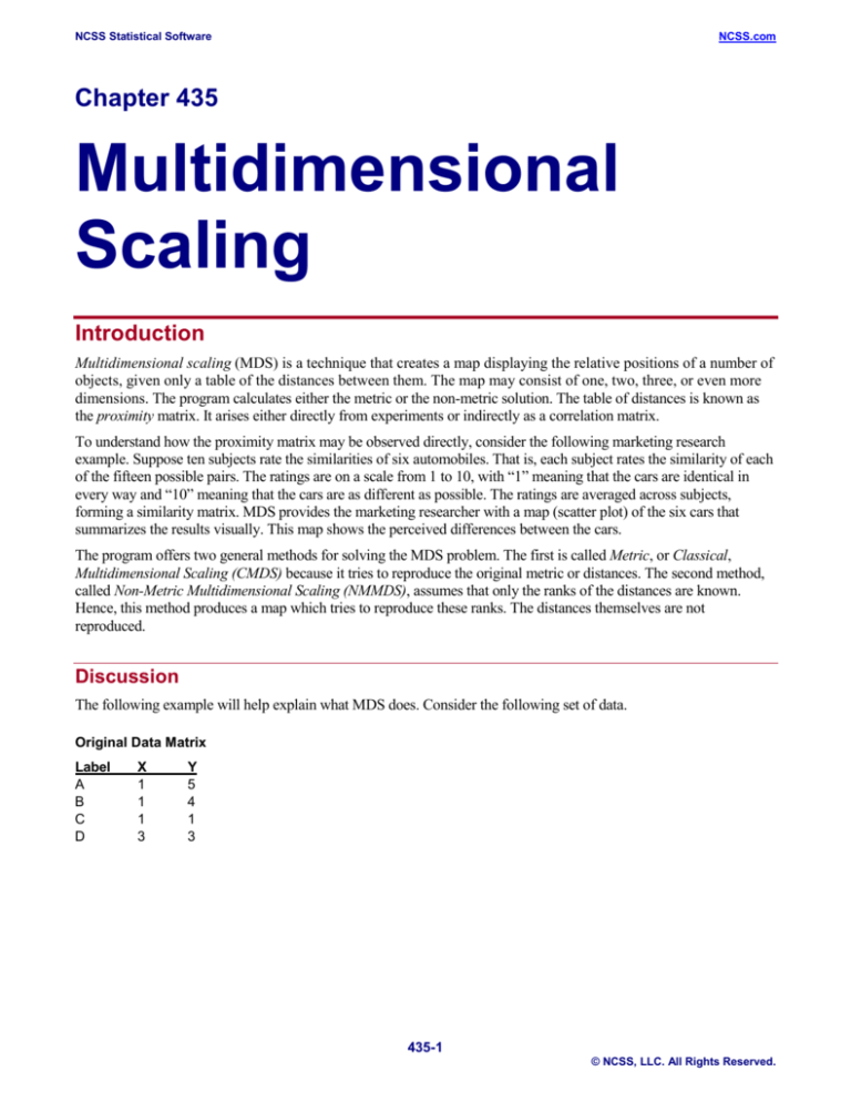
The following example will help explain what MDS does. Consider the following set of data.
Original Data Matrix
Label
A
B
C
D
X
1
1
1
3
Y
5
4
1
3
435-1
© NCSS, LLC. All Rights Reserved.
NCSS Statistical Software
NCSS.com
Multidimensional Scaling
A scatter plot of these data appears as follows:
6.0
X vs Y
4.5
A
D
1.5
Y
3.0
B
0.0
C
0.5
1.3
2.0
2.8
3.5
X
Notice that the scatter plot lets us visually assess the distance between each pair of points. We can see that A is near
B, but far from C and D. We can also see that C and D each seem to be by themselves. The actual distance between
two points i and j may be computed numerically using the Euclidean distance formula:
p
d ij =
∑(x
ik
− x jk
k =1
)
2
where p is the number of dimensions (which is 2 in our example), dij is the distance, and xik is the data value of the ith
row and kth column. This formula is an simple extension of the famous Pythagorean Theorem. Note that this formula
allows for an unlimited number of dimensions. That is, although we are only plotting the points in two-dimensional
space, the formula computes the distance in p-dimensional space, where p can be greater than two.
For example, the distance from A to D is calculated as follows:
2.82843 = (1 - 3 )2 + (5 - 3 )2 1
These distances are arranged in matrix format as follows:
Computed Distance Matrix
A
B
C
D
A
0.00000
1.00000
4.00000
2.82843
B
1.00000
0.00000
3.00000
2.23607
C
4.00000
3.00000
0.00000
2.82843
D
2.82843
2.23607
2.82843
0.00000
Note that since the distance from A to D is the same as the distance from D to A, the distance matrix is symmetric.
We only need to consider half of the matrix. In the program, we only require the upper half. The final distance matrix
will be:
Upper-Triangular Distance Matrix
A
B
C
D
A
0.00000
B
1.00000
0.00000
C
4.00000
3.00000
0.00000
D
2.82843
2.23607
2.82843
0.00000
The task attempted by MDS is that given only a distance matrix, find the original data so that a map (scatter plot) of
the data may be drawn.
Some of the difficulties facing MDS may be seen even in this simple example. First, as the number of objects
increases, the possible number of dimensions increases as well. If you have three objects, these will at most define a
435-2
© NCSS, LLC. All Rights Reserved.
NCSS Statistical Software
NCSS.com
Multidimensional Scaling
two-dimensional plane. With four objects, you will usually find a three-dimensional space. And so on, with each new
object adding one more possible dimension.
Also, notice that if the data are shifted in such a way that their positions relative to each other are maintained (rotated,
translated, or transposed), the computed distance matrix will be the same. Hence, the distance matrix could have come
from numerous sets of data.
A third challenge comes when the distances themselves are not actually known. You might only be given knowledge
of their relative size.
MDS techniques have proved useful because circumstances often occur where the actual coordinates of the objects
are not known, but some type of distance matrix is available. This is especially the case in psychology where people
cannot draw an overall picture of a group of objects, but they can express how different individual pairs of objects are.
From these pair-wise differences MDS often can provide a useful picture.
Goodness-of-Fit
As in any data analysis problem, an expression is needed to express how well a particular set of data are represented
by the model that the analysis imposes. In the case of MDS, you are trying to model the distances. Hence, the most
obvious choice for a goodness-of-fit statistic is one based on the differences between the actual distances and their
predicted values. Such a measure is called stress and is calculated as values:
stress =
∑ ( d − d )
∑d
ij
2
ij
2
ij
Here dij is predicted distance based on the MDS model. Note that this predicted value depends on the number of
dimensions kept and the algorithm that you used (metric versus non-metric).
As you can see from this equation, MDS fits with stress values near zero are the best.
In his original paper on MDS, Kruskal (1964) gave following advise about stress values based on his experience:
Stress
0.200
0.100
0.050
0.025
0.000
Goodness-of-fit
poor
fair
good
excellent
perfect
More recent articles caution against using a table like this since acceptable values of stress depends on the quality of
the distance matrix and the number of objects in that matrix.
Number of Dimensions
One of the main tasks the analyst has is determining the number of dimensions in the MDS model. Each dimension
represents a different underlying factor. One of the goals of the MDS analysis is to keep the number of dimensions as
small as possible. Usually, the analyst will anticipate select two or, at most, three dimensions. If more are required,
you may decide that MDS is not appropriate for your data.
The usual technique is to solve the MDS problem for a number of dimension values and adopt the smallest number of
dimensions that achieves a reasonably small value of stress. The program displays a simple bar chart of the stress
values to aid in the selection of the number of dimensions.
435-3
© NCSS, LLC. All Rights Reserved.
NCSS Statistical Software
NCSS.com
Multidimensional Scaling
Some researchers also consider the relative size of the eigenvalues that are generated during the solution process.
These eigenvalues are then used to determine the number of dimensions just as they are used in factor analysis to
determine the number of factors.
Proximity Measures
Proximity measures quantify how “close” two objects are. The program accepts three forms of proximity values:
dissimilarities, similarities, and correlations.
Dissimilarities represent the distance between two objects. They may be measured directly, as in the distance between
two towns, or approximated, as in “Bill is five points different from Joe on a ten-point scale.” MDS algorithms use the
dissimilarities directly. A dissimilarity matrix is symmetrical.
Similarities represent how close (in some sense) two objects are. The program lets you enter a similarity measure for
each pair of objects. Similarities must obey the rule: similarityij <= similarityii and similarityjj for all i and j. Similarity
matrices are symmetrical.
Similarities are converted to dissimilarities using the formula:
d ij = sii + s jj − 2sij
where d ij represents a dissimilarity and sij represents a similarity.
When your data consists of standard measures rather than dissimilarities or similarities, you can create a dissimilarity
matrix by first creating the correlation matrix and then using the above formula to convert the correlations to
dissimilarities. The program automatically calculates pair-wise correlations for the variable you specify.
Comparison of Metric and Non-Metric MDS
Although the computations are simpler for the metric method than for the non-metric method, both seem to yield
similar results when applied to well-known examples. When you have true distance data, the classical method yields a
solution that can be used directly. When you only have dissimilarities, the non-metric approach is somewhat more
appealing.
Metric MDS
Classical MDS procedures stem back to Torgerson (1952), who was one of the pioneers of the technique. His
algorithm is explained next.
Suppose a distance matrix D approximates the inter-point distances of a configuration of points X in a space of low
dimensionality p (usually p = 1, 2, or 3). That is, the elements of D, denoted d ij , may be calculated from X using the
following formula:
p
d ij =
∑(x
ik
k =1
− x jk
)
2
The steps in the classical MDS algorithm are as follows:
{
}
1. From D calculate A = − 12 d ij 2 .
{
}
2. From A calculate B = a ij − a i. − a. j + a.. , where a i. is the average of all a ij across j.
435-4
© NCSS, LLC. All Rights Reserved.
NCSS Statistical Software
NCSS.com
Multidimensional Scaling
3. Find the p largest eigenvalues λ 1 > λ 2 >  > λ p of B and corresponding eigenvectors
(
)
L = L(1) , L( 2) ,  L( p ) which are normalized so that L(′i ) L( i ) = λ i . (We are assuming that p is selected so that
the eigenvalues are all relatively large and positive.)
4. The coordinates of the objects are the rows of L.
The classical solution is optimal in the least-squares sense. That is, when a direct solution is possible (i.e., when D is
truly a Euclidean distance matrix), the solution, L, minimizes the sum of squared differences between the actual d ij ’s
(elements of D) and the d ’s based on L. Another way of saving this is that it minimizes the value of stress, where
ij
stress was defined above.
Non-Metric MDS
Implicit in the above is the assumption that there is a true configuration in p dimensions, i.e., that D is a distance
matrix. Often, however, it is more realistic to assume a less stringent relationship between the observed distances (or
dissimilarities) d ij and the true distances, denoted δ ij . That is, suppose we assume that
(
d ij = f δ ij + eij
)
where eij represents errors of measurements, distortions, etc. Also, we assume that f(x) is an unknown,
monotonically-increasing function.
For this model, the only information we can use is the rank order of the d ij . Usually, this approach is used when D is
simply a dissimilarity matrix rather than a true distance matrix. This assumption is often more plausible in practical
situations.
An algorithm to produce a solution based only on the rank order information was provided by Kruskal (1964). It is
involved, so we will not reproduce it here. We note that Kruskal’s algorithm minimizes stress.
Kruskal’s algorithm uses steepest descent to find a local minimum from a given starting configuration. The choice of
the starting configuration is important to finding the global rather than a local minimum. Many authors recommend
using the solution of the metric MDS as the starting configuration. This is the default starting configuration in this
program. You may also select several random starting configurations and compare the resulting stress values.
Data Structure
The data are may be entered in three formats. The first format is the standard row-column format from which the
correlations have be calculated. The MDS conducted on the correlations in an attempt to determine which of the
variables are similar. The second format is the upper-triangular portion of a distance matrix. The third format is
the upper-triangular portion of a similarity matrix.
An example of an upper-triangular distance matrix is contained in the MDS2 database. We suggest that you open
this database now so that you can follow along with the example.
435-5
© NCSS, LLC. All Rights Reserved.
NCSS Statistical Software
NCSS.com
Multidimensional Scaling
MDS2 dataset
Sport
Hockey
Football
Basketball
Tennis
Golf
Croquet
Hockey
0
Football
2
0
Basketball
3
3
0
Tennis
4
5
5
0
Golf
5
6
4
4
0
Croquet
5
5
6
3
2
0
Procedure Options
This section describes the options available in this procedure.
Variables Tab
This panel specifies the variables used in the analysis.
Input Variables
Input Variables
Specify the variables containing the upper-triangular distance, or similarity, matrix or the variables from which
the correlation matrix is to be calculated. Note that filter may not be used with the upper-triangular matrices.
Input Data Type
You can specify which of the three possible types of input data you have: dissimilarities, similarities, or
correlation.
Dissimilarities and similarities signal the program that an upper-triangular matrix is to be read in. When the
correlation option is selected, the program generates a correlation matrix from the standard variable by
observation data format that is used throughout the rest of the program.
Options
Solution Type
This option specifies whether you want the Metric or the Non-Metric algorithm used.
Options – Dimensions Reported
Minimum and Maximum Dimensions
These options specify a range of dimensions to be reported on. The MDS algorithm will be run on each of these
dimensions and the stress value will be calculated.
Dimensions Used
This option specifies the number of dimensions on which all results are based. This is the number of dimensions
that will be plotted.
435-6
© NCSS, LLC. All Rights Reserved.
NCSS Statistical Software
NCSS.com
Multidimensional Scaling
Options – Non-Metric MDS Options
Initial Configuration
This option specifies which starting configuration you want when using NMMDS. You can specify either
Random or Metric. We suggest the Metric option since it has been more widely recommend. You should only use
the Random option when the Metric option fails to produce good results.
Max Iterations/Dimension
This option specifies the maximum number of iterations run during the solution of a NMMDS problem for a
particular number of dimensions.
Max Iterations/Min Phase
This option specifies the maximum number of iterations run during minimization phase.
Min Stress Value
This option specifies the value of stress that must achieved in order to stop iterations during a run of NMMDS.
Min Stress Change
This option specifies the change in stress from one iteration to the next that must achieved in order to stop
iterations during a run of NMMDS.
Min Gradient Sum
This option specifies the value of the gradient sum that must achieved in order to stop iterations during a run of
NMMDS.
Reports Tab
The following options control which reports are displayed.
Select Reports
Eigenvalue Report - Dissimilarity Report
Specify whether to display the indicated report.
Report Options
Precision
Specify the precision of numbers in the report. Single precision will display seven-place accuracy, while double
precision will display thirteen-place accuracy.
Variable Names
This option lets you select whether to display variable names, variable labels, or both.
Plots Tab
These options control the attributes of the two plots.
Select Plots
MDS Map – Dissimilarity Plot
Specify whether to display the indicated plot. Click the plot format button to change the plot settings.
435-7
© NCSS, LLC. All Rights Reserved.
NCSS Statistical Software
NCSS.com
Multidimensional Scaling
Plot Options
Size of Plots
This option controls the size of the plots that are displayed. You can select small, medium, or large. Medium and
large are displayed one per line, while small are displayed two per line.
Storage Tab
Optionally specify columns to contain the coordinate values generated by the program.
Data Storage Columns
Coordinate Values
A list of columns into which the coordinate values (the values that are plotted) are stored.
Example 1 – Metric Multidimensional Scaling
This section presents an example of how to run an analysis of the data contained in the MDS2 dataset.
You may follow along here by making the appropriate entries or load the completed template Example 1 by
clicking on Open Example Template from the File menu of the Multidimensional Scaling window.
1
Open the MDS2 dataset.
•
From the File menu of the NCSS Data window, select Open Example Data.
•
Click on the file MDS2.NCSS.
•
Click Open.
2
Open the Multidimensional Scaling window.
•
On the menus, select Analysis, then Multivariate Analysis, then Multidimensional Scaling. The
Multidimensional Scaling procedure will be displayed.
•
On the menus, select File, then New Template. This will fill the procedure with the default template.
3
Specify the variables.
•
On the Multidimensional Scaling window, select the Variables tab.
•
Double-click in the Input Variables box. This will bring up the variable selection window.
•
Select Hockey to Croquet from the list of variables and then click Ok. “Hockey-Croquet” will appear in
the Input Variables box.
4
Run the procedure.
•
From the Run menu, select Run Procedure. Alternatively, just click the green Run button.
435-8
© NCSS, LLC. All Rights Reserved.
NCSS Statistical Software
NCSS.com
Multidimensional Scaling
Eigenvalue Section
Eigenvalue Section
Dim
No.
Eigenvalue
1
30.73
2 (Used)
12.85
3
6.38
4
1.68
5
0.00
6
-4.98
Total
56.62
Individual
Percent
54.28
22.69
11.27
2.97
0.00
8.79
Cumulative
Percent
54.28
76.97
88.24
91.21
91.21
100.00
Bar Chart
|IIIIIIIIIIIIIIIIIIIIIIIIIII
|IIIIIIIIIII
|IIIIII
|I
|
|IIII
This report is produced by CMDS.
In this particular example, the first two dimensions account for 77% of the variation while the first three
dimensions account for 88%. We would probably use two or perhaps three dimensions.
Eigenvalues
These are the eigenvalues found during CMDS. The eigenvalues are helpful in determining the number of
dimensions that are necessary to represent the dissimilarity matrix accurately. As in factor analysis, the task is to
select enough dimensions to approximate the data, but few enough to keep the interpretation simple. The
eigenvalue report allows you to quickly determine the impact of each new dimension.
In MDS, some of the eigenvalues can be negative. Do not keep these dimensions. The basic rule is to find the
number of relatively large, positive eigenvalues. This report provides a bar graph and percentages to help you
determine the number of dimensions.
Individual and Cumulative Percents
The first column gives the percentage of the total of the absolute value of the eigenvalues accounted for by this
dimension. The second column is the cumulative total of the percentage.
Bar Chart
This is a rough bar plot of the eigenvalues. It enables you to quickly note the relative size of each eigenvalue.
Many authors recommend it as a method of determining how many dimensions to retain.
Fit Summary Section
Fit Summary Section (Metric Solution)
No.
Dim's
1
2
3
4
Squared
Differences
37.105982
6.947666
2.413305
2.468686
Stress
0.364035
0.157522
0.092838
0.093897
Pseudo
R-Squared
0.00
70.73
89.83
89.60
Number of Dissimilarities
Mean of Dissimilarities
Sum of Squared Dissimilarities
Mean Corrected Sum of Squared Dissimilarities
15
4.133333
280.000000
23.733333
This report provides information useful in determining the number of dimensions that are necessary and assessing
the goodness-of-fit of the CMDS model.
No. Dim’s
The number of dimensions used in calculating this row of statistics.
435-9
© NCSS, LLC. All Rights Reserved.
NCSS Statistical Software
NCSS.com
Multidimensional Scaling
Squared Differences
The sum of the squared differences between the actual dissimilarity values and those predicted by the solution.
Stress
This is the value of the stress goodness-of-fit statistic. It is equal to the square root of the Squared Differences
divided by the square root of the Sum of the Squared Dissimilarities. It is one of the most popular measures of
accuracy of the fit. A value below 0.05 is acceptable. A value below 0.01 is considered good.
Pseudo R-Squared
This is an index, similar to the R-squared value in regression analysis, which indicates what percentage of the sum
of squared dissimilarities (corrected for the mean) is accounted for by this number of dimensions. A value above
80% is hoped for.
Number of Dissimilarities
This is the number of dissimilarity values.
Mean of Dissimilarities
This is the mean of the dissimilarity values
Sum of Squared Dissimilarities
This is the sum of the squared dissimilarities. It is the denominator of the stress statistic.
Mean Corrected Sum of Squared Dissimilarities
This is the sum of the squared dissimilarities about their mean. It is the denominator of the Pseudo R-Squared
statistic.
Solution Section
Solution Section
Variables
Hockey
Football
Basketball
Tennis
Golf
Croquet
Dim1
1.9301
2.6179
2.1119
-1.4786
-2.3836
-2.7976
Dim2
-0.6756
-1.1281
2.0914
-1.3608
2.0059
-0.9328
Dim3
0.3818
-1.1303
0.4168
1.8070
-0.2743
-1.2011
Dim4
1.0441
-0.4680
-0.4032
-0.3940
0.2351
-0.0140
This report presents the solution of the MDS procedure. These are the data that are plotted in the MDS map. They
have been scaled so that the sum of squares for each column is equal to the eigenvalue for that dimension.
Note that these data were constructed so that the distance between two rows is close to the original dissimilarity
value.
Although some interpretation of these numbers may be made directly, usually the data are displayed on scatter
plots.
435-10
© NCSS, LLC. All Rights Reserved.
NCSS Statistical Software
NCSS.com
Multidimensional Scaling
Dissimilarity Section
Dissimilarity Section
Row
1 Hockey
5 Golf
2 Football
4 Tennis
1 Hockey
1 Hockey
3 Basketball
4 Tennis
2 Football
3 Basketball
2 Football
1 Hockey
1 Hockey
3 Basketball
2 Football
Actual
Predicted
Column
Dissimilarity Dissimilarity
2 Football
2.000000
0.823324
6 Croquet
2.000000
2.967759
3 Basketball
3.000000
3.259039
6 Croquet
3.000000
1.386718
3 Basketball
3.000000
2.772988
4 Tennis
4.000000
3.476854
5 Golf
4.000000
4.496329
5 Golf
4.000000
3.486229
6 Croquet
5.000000
5.419049
4 Tennis
5.000000
4.980893
4 Tennis
5.000000
4.103106
6 Croquet
5.000000
4.734691
5 Golf
5.000000
5.079231
6 Croquet
6.000000
5.766223
5 Golf
6.000000
5.902321
Dimensions
Sum of Squared Dissimilarities
Sum of Squared Differences
Stress
Pseudo R-Squared
Actual
Difference
1.176676
-0.967759
-0.259039
1.613282
0.227012
0.523146
-0.496329
0.513771
-0.419049
0.019107
0.896894
0.265309
-0.079231
0.233777
0.097679
Percent
Difference
58.83
-48.39
-8.63
53.78
7.57
13.08
-12.41
12.84
-8.38
0.38
17.94
5.31
-1.58
3.90
1.63
2
280.000000
6.947666
0.157522
70.726127
You might think of this as a residual analysis report since it highlights the differences between the actual and the
predicted dissimilarities. It will let you focus on those dissimilarities that are not fit well by the model.
Row
The variable associated with this row of the dissimilarity matrix.
Column
The variable associated with this column of the dissimilarity matrix.
Actual Dissimilarity
The value from the input (or calculated) dissimilarity matrix for this row and column.
Predicted Dissimilarity
The predicted dissimilarity value based on the number of dimensions that you have selected.
Actual Difference
The Actual Dissimilarity minus the Predicted Dissimilarity. This value shows the size of the error in predicting
this element of the dissimilarity matrix.
Percent Difference
The percentage the Actual Difference is of the Actual Dissimilarity. This value highlights the outliers--those
dissimilarities that are not fit well by the MDS model.
Dimensions
The number of dimensions used in calculating the statistics.
Sum of Squared Dissimilarities
This is the sum of the squared dissimilarities. It is the denominator of the stress statistic.
Sum of Squared Differences
This is the sum of the squared differences. It is the numerator of the stress statistic.
435-11
© NCSS, LLC. All Rights Reserved.
NCSS Statistical Software
NCSS.com
Multidimensional Scaling
Stress
This is the value of the stress goodness-of-fit statistic. It is equal to the Squared Differences divided by the Sum of
the Squared Dissimilarities. It is one of the most popular measures of accuracy of the fit. A value below 0.05 is
acceptable. A value below 0.01 is considered good.
Pseudo R-Squared
This is an index, similar to the R-squared value in regression analysis, which indicates what percentage of the sum
of squared dissimilarities (corrected for the mean) is accounted for by this number of dimensions. A value above
80% is hoped for.
MDS Map
This plot is the chief objective of an MDS analysis. It is often referred to as the MDS map. It allows you to
interpret the dissimilarity matrix on a two-dimensional scatter plot.
There is no real orientation to this map. You could legitimately rotate the values around the plot’s center. The
main characteristics of interest are the relative positions of the points and any clusters that are apparent.
In this example, we see that the respondents considered hockey and football to be similar. They also considered
croquet and tennis to be quite similar. Football appears quite different from golf. And so on. Notice how easy it is
to draw conclusions about the similarities among the sports.
A second task of the MDS analyst is to find the underlying factors that respondents used when they created these
dissimilarities. For example, a vertical line down the center of the plot would divide team sports on the right from
individual sports on the left. We would hypothesize this as one interpretation of the Dim1 (horizontal) axis.
435-12
© NCSS, LLC. All Rights Reserved.
NCSS Statistical Software
NCSS.com
Multidimensional Scaling
Example 2 – Non-Metric Multidimensional Scaling
This section presents an example of how to run an analysis of the data contained in the MDS2 dataset using
NMMDS.
You may follow along here by making the appropriate entries or load the completed template Example 2 by
clicking on Open Example Template from the File menu of the Multidimensional Scaling window.
1
Open the MDS2 dataset.
•
From the File menu of the NCSS Data window, select Open Example Data.
•
Click on the file MDS2.NCSS.
•
Click Open.
2
Open the Multidimensional Scaling window.
•
On the menus, select Analysis, then Multivariate Analysis, then Multidimensional Scaling. The
Multidimensional Scaling procedure will be displayed.
3
Specify the variables.
•
On the Multidimensional Scaling window, select the Variables tab.
•
Double-click in the Input Variables box. This will bring up the variable selection window.
•
Select Hockey to Croquet from the list of variables and then click Ok. “Hockey-Croquet” will appear in
the Input Variables box.
•
Enter Non-Metric in the Solution Type box.
4
Run the procedure.
•
From the Run menu, select Run Procedure. Alternatively, just click the green Run button.
Eigenvalue Section
Eigenvalue Section
Dim
No.
Eigenvalue
1
30.73
2 (Used)
12.85
3
6.38
4
1.68
5
0.00
6
-4.98
Total
56.62
Individual
Percent
54.28
22.69
11.27
2.97
0.00
8.79
Cumulative
Percent
54.28
76.97
88.24
91.21
91.21
100.00
Bar Chart
|IIIIIIIIIIIIIIIIIIIIIIIIIII
|IIIIIIIIIII
|IIIIII
|I
|
|IIII
This report is produced by CMDS which was used as the starting configuration. Its definitions were given above
and will not be repeated here.
Non-Metric Iteration Summary Section
Non-Metric Iteration Summary Section
No.
Percent Rank
Dim's
Maintained
Stress
1
57.14
0.212628
2
64.29
0.052276
3
78.57
0.000344
4
64.29
0.000003
Why
Terminated
Stress Change
Stress Change
Max Iterations
Min Stress
Bar Chart
of Stress
|IIIIIIIIIIIIIIIIIIIIIIIIIIIIIIIIIIIIIIIIIIIIIIII<<I
|IIIIIIIIIIIIIIIIIIIIIIIIII
|
|
This report provides information about the number of dimensions that are necessary and the goodness-of-fit of the
solution.
435-13
© NCSS, LLC. All Rights Reserved.
NCSS Statistical Software
NCSS.com
Multidimensional Scaling
No. Dim’s
The number of dimensions used in calculating this row of statistics.
Percent Rank Maintained
The non-metric solution tries to maintain the rank ordering of the dissimilarities. This is the percentage of the
dissimilarities whose rank order was maintained. The higher this value is, the better the quality of the solution.
Stress
Defined earlier, this is one of the most popular measures of accuracy of the fit. A value below 0.05 is acceptable.
A value below 0.01 is considered good.
Why Terminated
This field explains which stopping rule caused the iterative procedure to stop. This is important to watch since the
solution is not optimal if the maximum iterations were reached before the algorithm converged. When this
happens, you should change some of the iteration control parameters, especially the number of iterations.
Bar Chart of Stress
This column graphically portrays the stress values. You want to choose the fewest number of dimensions that give
you a small stress value.
Solution Section
Solution Section
Variables
Hockey
Football
Basketball
Tennis
Golf
Croquet
Dim1
0.3306
0.4234
0.2674
-0.2542
-0.3473
-0.4199
Dim2
-0.1495
-0.0227
0.2837
-0.3538
0.2227
0.0196
This report presents the final configuration of the NMMDS procedure. These are the data that are plotted in the
MDS map.
Note that these data were not constructed so that the distance between two rows is close to the original
dissimilarity value. Instead, the non-metric solution attempts to maintain the same rank ordering of the calculated
distances as occur in the original dissimilarity matrix. Although some interpretation of these numbers may be
made directly, usually the data are displayed on scatter plots.
435-14
© NCSS, LLC. All Rights Reserved.
NCSS Statistical Software
NCSS.com
Multidimensional Scaling
Dissimilarity Section
Dissimilarity Section
Row
5 Golf
1 Hockey
2 Football
4 Tennis
1 Hockey
1 Hockey
3 Basketball
4 Tennis
2 Football
3 Basketball
2 Football
1 Hockey
1 Hockey
2 Football
3 Basketball
Actual
Predicted
Column
Dissimilarity Dissimilarity
6 Croquet
2.000000
0.215646
2 Football
2.000000
0.157123
3 Basketball
3.000000
0.343893
6 Croquet
3.000000
0.408445
3 Basketball
3.000000
0.437798
4 Tennis
4.000000
0.619391
5 Golf
4.000000
0.617695
5 Golf
4.000000
0.583869
6 Croquet
5.000000
0.844336
4 Tennis
5.000000
0.823650
4 Tennis
5.000000
0.754122
6 Croquet
5.000000
0.769237
5 Golf
5.000000
0.773283
5 Golf
6.000000
0.808819
6 Croquet
6.000000
0.736258
You might think of this as a residual analysis report since it highlights the differences between the actual and the
predicted dissimilarities. It will let you focus on those dissimilarities that are not fit well by the model.
This report presents the details of how well the rank ordering of the dissimilarity values is preserved in the final
configuration. Note that the predicted values are quite different from the actual values since all the algorithm was
attempting to do was maintain the ordering.
Row
The variable associated with this row of the dissimilarity matrix.
Column
The variable associated with this column of the dissimilarity matrix.
Actual Dissimilarity
The value from the input (or calculated) dissimilarity matrix for this row and column.
Predicted Dissimilarity
The predicted dissimilarity value based on the number of dimensions that you have selected. Note that this is not
predicting the actual dissimilarity value, but some unknown function of the dissimilarity value. It is not usually necessary
to determine the function. We are mainly interested in how well the ordering of the actual values is maintained by these
predicted values.
435-15
© NCSS, LLC. All Rights Reserved.
NCSS Statistical Software
NCSS.com
Multidimensional Scaling
MDS Map
This plot is the chief objective of an MDS analysis. It is often referred to as the MDS map. It allows you to
interpret the dissimilarity matrix on a two-dimensional scatter plot.
There is no real orientation to this map. You could legitimately rotate the values around the plot’s center. The
main characteristics of interest are the relative positions of the points and any clusters that are apparent.
In this example, we see that the respondents considered hockey and football to be similar. They also considered
croquet and golf to be similar. Football appears quite different from croquet. And so on. Notice how easy it is to
draw conclusions about the similarities among the sports.
A second task of the MDS analyst is to find the underlying factors that respondents used when they created these
dissimilarities. For example, a vertical line down the center of the plot would divide team sports on the right from
individual sports on the left. We might hypothesize this as one interpretation of the Dim1 (horizontal) axis.
It is interesting to compare this map with the map produced by the metric solution. The main difference appears to
be that golf and croquet are now much closer together (as they were rated in the original data). Again, football and
basketball appear to be closer together in this plot as we might expect from the original data. In this case, the
NMMDS map appears to be more accurate than the CMDS map. This is as we might expect since, the NMMDS
procedure refined the CMDS map.
435-16
© NCSS, LLC. All Rights Reserved.
NCSS Statistical Software
NCSS.com
Multidimensional Scaling
Dissimilarity Fit Plot
This graph plots the dissimilarity values on the vertical axis against the predicted dissimilarity values on the
horizontal axis. The caliber of the solution depends upon this plot showing an upward-sloping trend. If the solution
was perfect, then as you move across the plot from left to right, you would never go down from one point to the
next.
We notice in this case that the solution confuses the large distances. This may be due to the large number of ties in
this area (look at the Dissimilarity Section to see all the 5’s and 6’s).
435-17
© NCSS, LLC. All Rights Reserved.