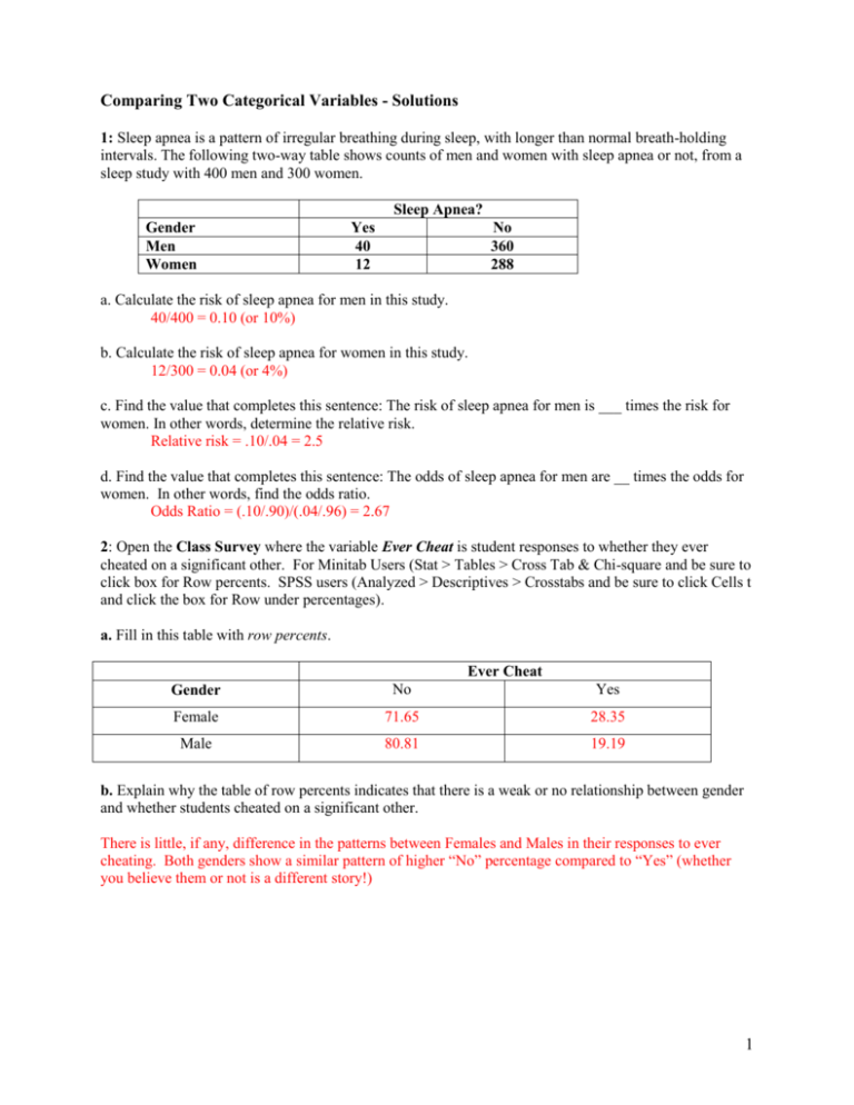
Comparing Two Categorical Variables - Solutions
1: Sleep apnea is a pattern of irregular breathing during sleep, with longer than normal breath-holding
intervals. The following two-way table shows counts of men and women with sleep apnea or not, from a
sleep study with 400 men and 300 women.
Sleep Apnea?
Gender
Men
Women
Yes
40
12
No
360
288
a. Calculate the risk of sleep apnea for men in this study.
40/400 = 0.10 (or 10%)
b. Calculate the risk of sleep apnea for women in this study.
12/300 = 0.04 (or 4%)
c. Find the value that completes this sentence: The risk of sleep apnea for men is ___ times the risk for
women. In other words, determine the relative risk.
Relative risk = .10/.04 = 2.5
d. Find the value that completes this sentence: The odds of sleep apnea for men are __ times the odds for
women. In other words, find the odds ratio.
Odds Ratio = (.10/.90)/(.04/.96) = 2.67
2: Open the Class Survey where the variable Ever Cheat is student responses to whether they ever
cheated on a significant other. For Minitab Users (Stat > Tables > Cross Tab & Chi-square and be sure to
click box for Row percents. SPSS users (Analyzed > Descriptives > Crosstabs and be sure to click Cells t
and click the box for Row under percentages).
a. Fill in this table with row percents.
Ever Cheat
Gender
No
Yes
Female
71.65
28.35
Male
80.81
19.19
b. Explain why the table of row percents indicates that there is a weak or no relationship between gender
and whether students cheated on a significant other.
There is little, if any, difference in the patterns between Females and Males in their responses to ever
cheating. Both genders show a similar pattern of higher “No” percentage compared to “Yes” (whether
you believe them or not is a different story!)
1
c. Perform a Chi-square test for statistical significance of independence of the observed relationship. For
Minitab Users (Repeat steps above but also click tab for Chi-square and select box for Chi-square
analysis. SPSS users (Repeat steps above but also click tab for Statistics and select box for Chi-square).
(i) Give Pearson p-value for the test,
Pearson Chi-Square = 2.532, DF = 1, P-Value = 0.112
(ii) explain whether the observed relationship is statistically significant and
The observed relationship is not significant since the p-value is greater than 0.05. We call this
“0.05” the alpha-level and we commonly use it as the critical value to which we compare the p-value. If
p-value ≤ alpha, we will say that the result is statistically significant, but if p-value is > alpha we will say
that we do not have enough evidence to support a statistically significant conclusion.
(iii) state a general conclusion. The conclusion is simply a summary statement. For this problem
our summary would be that based on our data there appears to be no significant relationship between
Gender and Cheating.
Minitab Output:
Tabulated statistics: Gender, EverCheat
Rows: Gender
Columns: EverCheat
No
Yes
All
Female
91
71.65
36
28.35
127
100.00
Male
80
80.81
19
19.19
99
100.00
All
171
75.66
55
24.34
226
100.00
Cell Contents:
Count
% of Row
Pearson Chi-Square = 2.532, DF = 1, P-Value = 0.112
SPSS Output:
Gender * EverCheat Crosstabulation
EverCheat
No
Count
Total
Yes
91
36
127
71.7%
28.3%
100.0%
80
19
99
80.8%
19.2%
100.0%
171
55
226
75.7%
24.3%
100.0%
Female
% within Gender
Gender
Count
Male
% within Gender
Count
Total
% within Gender
2
Chi-Square Tests
Value
Pearson Chi-Square
Continuity
Correctionb
Likelihood Ratio
df
Asymp. Sig. (2-
Exact Sig. (2-
Exact Sig. (1-
sided)
sided)
sided)
2.532a
1
.112
2.059
1
.151
2.572
1
.109
Fisher's Exact Test
N of Valid Cases
.121
.075
226
a. 0 cells (0.0%) have expected count less than 5. The minimum expected count is 24.09.
b. Computed only for a 2x2 table
3 The High School and Beyond study is from a large-scale longitudinal study conducted by the
National Opinion Research Center under contract with the National Center for Education
Statistics. Below is a table (note: this is called summarized data!) representing a sample of
100 students from this data that includes the student’s gender and whether the high school they
attended was public or private. Perform a Chi-square analysis of independence for this data. For
Minitab and SPSS users you will first need to enter this data into your worksheet. [Special Note:
Recall from the probability lesson this would be a test of independence: that is, can we say that
the probability of being Female is independent of the probability that school type is public?]
Minitab users: you can just enter the counts as displayed below with 38 and 46 being in the first
two cells of C1 and 7 and 9 being in the first two cells of C2. For Minitab users (Stat > Tables >
Table in Worksheet)
SPSS users: after opening SPSS you need to enter the counts in first column (e.g. 38, 46, 7, 9),
then in second column type in Female or Male depending on which gender the number relates to
(e.g. Female, Male, Female, Male) and make sure you spell each correctly and using
consistent casing, i.e. capitalization. Finally in third column type in school type for that count
(note SPSS defaults to 6 letters) (e.g. Pu, Pu, Pr, Pr). Then go to Data > Weight cases > click
radio button for Weight cases and enter the column containing the counts. Now do chi—square
test by Analyze > Descriptives > Crosstabs.
Female
Male
Total
(i)
Public
38
46
84
Private
7
9
16
Total
45
55
100
include a relevant table of conditional percents,
3
Public
84.4%
83.6%
Female
Male
Total
(ii)
(iii)
(i)
(ii)
(iii)
Private
15.6%
16.4%
Total
based on the percents, discuss the nature of any relationship, and
do a chi-square test of statistical significance. State a clear conclusion for the test of
significance.
The relevant table is shown above with the row percent given below the cell count.
For example, the 7 females from private school account for 15.6% of the total
females.
There appears to be no relationship between Gender and School Type as there is not a
large difference in the row percents between the Genders for either school type.
The p-value (0.913) is greater than 0.05 indicating NO statistically significant
relationship. We would conclude, then, that our data does not show a statistically
significant relationship between Gender and School Type. [NOTE: this would mean
that Gender and School Type are independent – similar to the probability activity].
Minitab Output: (note: the output was edited to include row and column names).
Tabulated statistics: Gender, School
Rows: Gender
Columns: School
Public
Private
All
Female
38
84.44
7
15.56
45
100.00
Male
46
83.64
9
16.36
55
100.00
All
84
84.00
16
16.00
100
100.00
Cell Contents:
Count
% of Row
Pearson Chi-Square = 0.012, DF = 1, P-Value = 0.913
SPSS Output:
VAR00002 * VAR00003 Crosstabulation
VAR00003
Priv
Count
Total
Public
7
38
45
15.6%
84.4%
100.0%
9
46
55
16.4%
83.6%
100.0%
16
84
100
16.0%
84.0%
100.0%
Female
% within VAR00002
VAR00002
Count
Male
% within VAR00002
Count
Total
% within VAR00002
4
Chi-Square Tests
Value
Pearson Chi-Square
Continuity
df
Asymp. Sig. (2-
Exact Sig. (2-
Exact Sig. (1-
sided)
sided)
sided)
.012a
1
.913
.000
1
1.000
.012
1
.913
Correctionb
Likelihood Ratio
Fisher's Exact Test
N of Valid Cases
1.000
.568
100
a. 0 cells (0.0%) have expected count less than 5. The minimum expected count is 7.20.
b. Computed only for a 2x2 table
4: Suppose a newspaper article states that drinking three or more cups of coffee doubles the risk
of gall bladder cancer. Before giving up coffee, what question should be asked by a person who
drinks this much coffee? (There is more than one possible answer.)
Some of these include:
Q. Is there a hereditary factor that was included in the study?
Q. What role did gender play?
Q. How was the data gathered and what was the sample size?
Q. What was the make-up of the data set? E.g. dispersion of age, gender.
Q. Is there a time factor? For instance, do you have to drink three or more cups of coffee for so
long before being at risk?
Q. Most importantly, this only shows a relationship and not a cause. So is there further info on
whether this behavior will cause gall bladder cancer?
5