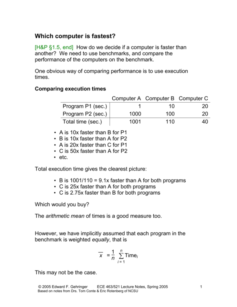
Which computer is fastest?
[H&P §1.5, end] How do we decide if a computer is faster than
another? We need to use benchmarks, and compare the
performance of the computers on the benchmark.
One obvious way of comparing performance is to use execution
times.
Comparing execution times
Computer A Computer B Computer C
Program P1 (sec.)
1
10
20
Program P2 (sec.)
1000
100
20
Total time (sec.)
1001
110
40
•
•
•
•
•
A is 10x faster than B for P1
B is 10x faster than A for P2
A is 20x faster than C for P1
C is 50x faster than A for P2
etc.
Total execution time gives the clearest picture:
• B is 1001/110 = 9.1x faster than A for both programs
• C is 25x faster than A for both programs
• C is 2.75x faster than B for both programs
Which would you buy?
The arithmetic mean of times is a good measure too.
However, we have implicitly assumed that each program in the
benchmark is weighted equally, that is
1
x =n
n
 Timei
i=1
This may not be the case.
© 2005 Edward F. Gehringer
ECE 463/521 Lecture Notes, Spring 2005
Based on notes from Drs. Tom Conte & Eric Rotenberg of NCSU
1
Suppose we have the following weightings:
Program 1 is run 80% of the time.
Program 2 is run 20% of the time.
Now which computer is fastest?
For Computer A, the mean is
For Computer B, the mean is
For Computer C, the mean is
Suppose we have these weightings:
Program 1 is run 99% of the time.
Program 2 is run 1% of the time.
Now which computer is fastest?
For Computer A, the mean is
For Computer B, the mean is
For Computer C, the mean is
When comparing weighted benchmarks, we must use this formula:
n
x =
 Weighti  Timei
i=1
So far, we have been comparing execution times. This seems pretty
natural.
But suppose that we express run times as “so many times the run
time on a reference machine.”
Why would we want to do this?
Let’s consider the execution times normalized to Computers A, B,
and C.
Lecture 3
Advanced Microprocessor Design
2
Normalized to A
A
B
C
Normalized to B
A
B
0.1
1.0
Normalized to C
C
A
B
C
0.05
0.5
1.0
Program P1
1.0 10.0
Program P2
1.0
0.1
10.0
1.0
50.0
5.0
1.0
Arith. mean
1.0 5.05
5.05
1.0
25.0 2.75
1.0
Geom.mean
1.0
1.0
1.0
1.58 1.58
1.0
1.0
Clearly, the arithmetic mean of normalized run times does not help
us decide which computer is fastest.
Geometric means
For normalized run times, we might instead use the geometric mean,
defined as
n n
 Execution time ratioi
i=1
The geometric means are consistent independent of normalization.
Comparing execution rates
Let’s now consider the situation where we want to compare execution
rates instead of execution times. Here our performance is expressed
not in time (time per program), but rather by rate (e.g., instructions
per unit time).
Prog 1
Prog 2
Harmonic mean
Arithmetic mean
Which is faster, A or B?
A
4
4
4
4
B
2
7
3.11
4.5
(Rates are given in instructions
per second)
Consider running an average instruction from Prog. 1 followed by one
from Prog. 2:
for A:
© 2005 Edward F. Gehringer
ECE 463/521 Lecture Notes, Spring 2005
Based on notes from Drs. Tom Conte & Eric Rotenberg of NCSU
3
for B:
runs the two instructions faster (1/2 < 9/14), thus is better.
What have we done? We have converted the rates to times, and
chosen the computer with the lower value.
For a measure that expresses this, we use the harmonic mean:
H =
N
n

1
ratei
i=1
The harmonic mean says A has a higher rate than B (4 vs. 3.11) so
The arithmetic mean says B has a higher rate than A (4.5 vs. 4) so B
is better, but that’s wrong!
If you used the wrong method to combine the numbers, you would
buy the slower machine!
Note also that the definition of harmonic mean is just the average of
the rates converted to times, then converted back to rates.
If the programs have different weights in the benchmark, we should
use this definition:
 n
 –1


H =   Weighti ÷ Ratei

i = 1
Rules
Use the arithmetic mean to combine run times.
Use the geometric mean to combine relative run times.
Use the harmonic mean to combine rates (e.g., IPC), because it
actually combines them as times then
converts back to a rate
die
defects
Cost of an Integrated Circuit
Lecture 3
Advanced Microprocessor Design
4
wafer
[H&P §1.4] Why do we care about the cost of integrated circuits in
this course?
To manufacture an integrated circuit, a wafer is tested and chopped
into dies.
Thus, the cost of a packaged IC is
Cost of IC =
Cost of die + Cost of testing die + Cost of packaging
Final test yield
If we knew how many dies (or “dice”) fit on a wafer, and how many of
them worked, then we could predict the cost of an individual die:
Cost of wafer
Cost of die = Dies per wafer x Die yield
area of wafer
The number of dies per wafer is basically the area of die .
But it is not exactly that, because
A more accurate estimate can be obtained by
Dies per wafer =
 
Wafer diameter2

2

Die area
–
 (wafer diameter)
2 x Die area
The second term compensates for the problem of a “square peg in a
round hole.”
Dividing the circumference by the diagonal of a square die is
approximately the number of dies along the edge.
For example, on the 8-inch wafer of MIPS64 R20K processors shown
in the text, how many 1-cm dies would we have?
© 2005 Edward F. Gehringer
ECE 463/521 Lecture Notes, Spring 2005
Based on notes from Drs. Tom Conte & Eric Rotenberg of NCSU
5
What else do we need to know to determine the cost of an integrated
circuit?
A simple empirical model of integrated circuit yield, which assumes
 that defects are randomly distributed over the wafer, and
 that yield is inversely proportional to the fabrication process
gives—

Die yield = Wafer yield  1 +
Defects per unit area x Die area –




According to the text,
 defects per unit area range between 0.4 and 0.8 per
square centimeter, and
 , a parameter that corresponds inversely to the number of
masking levels, is approximately 4.0.
This gives a die yield of about 0.57 for dies that are 1 cm. on a side.
In today’s computers, the most expensive parts are the processor
and the monitor, each accounting for about 20% of the price.
Moore’s Law
In 1965, Gordon Moore of Fairchild Semiconductor, who went on to
co-found Intel, observed that that the number of transistors per
square inch on integrated circuits had doubled every year since the
integrated circuit was invented.
Moore predicted that this trend would continue for the foreseeable
future.
Lecture 3
Advanced Microprocessor Design
6
Here is a table that shows transistor counts for Intel processors:
Processor
4004
8008
8080
8086
286
386™ processor
486™ DX processor
Pentium® processor
Pentium II processor
Pentium III processor
Pentium 4 processor
Itanium® processor
Itanium 2 processor
Year
1971
1972
1974
1978
1982
1985
1989
1993
1997
1999
2000
2002
2003
Transistor count
2,250
2,500
5,000
29,000
120,000
275,000
1,180,000
3,100,000
7,500,000
24,000,000
42,000,000
220,000,000
410,000,000
(Source: http://www.intel.com/research/silicon/mooreslaw.htm)
Although the number of transistors/in2 has not doubled quite that fast,
data density has doubled approximately every 18 months.
This is the current definition of Moore's Law, which Moore himself
has blessed.
Another way of stating this: Computing performance doubles every
18 months, for equal cost.
Buy first computer today, then buy a second computer at the same
price 18 months from now. Second computer is twice as fast
Moore’s Law speedup equation:
perf(m months from now) = 2m /18  perf(now)
or
perf(y years from now) =
How would we express speedup of the new machine vs. the old?
© 2005 Edward F. Gehringer
ECE 463/521 Lecture Notes, Spring 2005
Based on notes from Drs. Tom Conte & Eric Rotenberg of NCSU
7
Speedup =
The Von Neumann Gap
Processor speed has increase far faster than memory speed. The
gap has now reached two orders of magnitude.
This means that a processor will not be able to run at full speed if it
always needs to fetch data from memory.
Let us assume that
 memory access speed is 60 ns.
 cycle time (CT) is 2 ns.
 CPI = 1 (not including cycles waiting for memory).
 Average # of memory accesses per instruction = 1.5. This
assumes—
all instructions are read from memory
half the instructions access data from memory
Now, as we saw in the last lecture, CPU time = IC  CPI  CT.
For an instruction count (IC) of 106,
CPU time = 106  1 + 1.5 2   2 ns. = 92  10–3 sec.
60
However, if we could make memory run at the speed of the CPU,
CPU time = 106  1 + 1.5 2  2 ns. = 5  10–3 sec.
2
There are memory technologies that will achieve this speed. Why
don’t we use them?
However, we can arrange to put the data that we need into fast
memory. We take advantage of two kinds of locality.

Lecture 3
Advanced Microprocessor Design
8

Here is a diagram of the caches in a modern computer system.
Registers
load
store
Data
Instruction
cache
cache
L1 caches
Cache miss
Unified data & instruction
L2 cache
"On board"
Cache miss
Memory bus
Physical memory
(e.g., SIMMs)
Page fault
Disk
© 2005 Edward F. Gehringer
ECE 463/521 Lecture Notes, Spring 2005
Based on notes from Drs. Tom Conte & Eric Rotenberg of NCSU
9