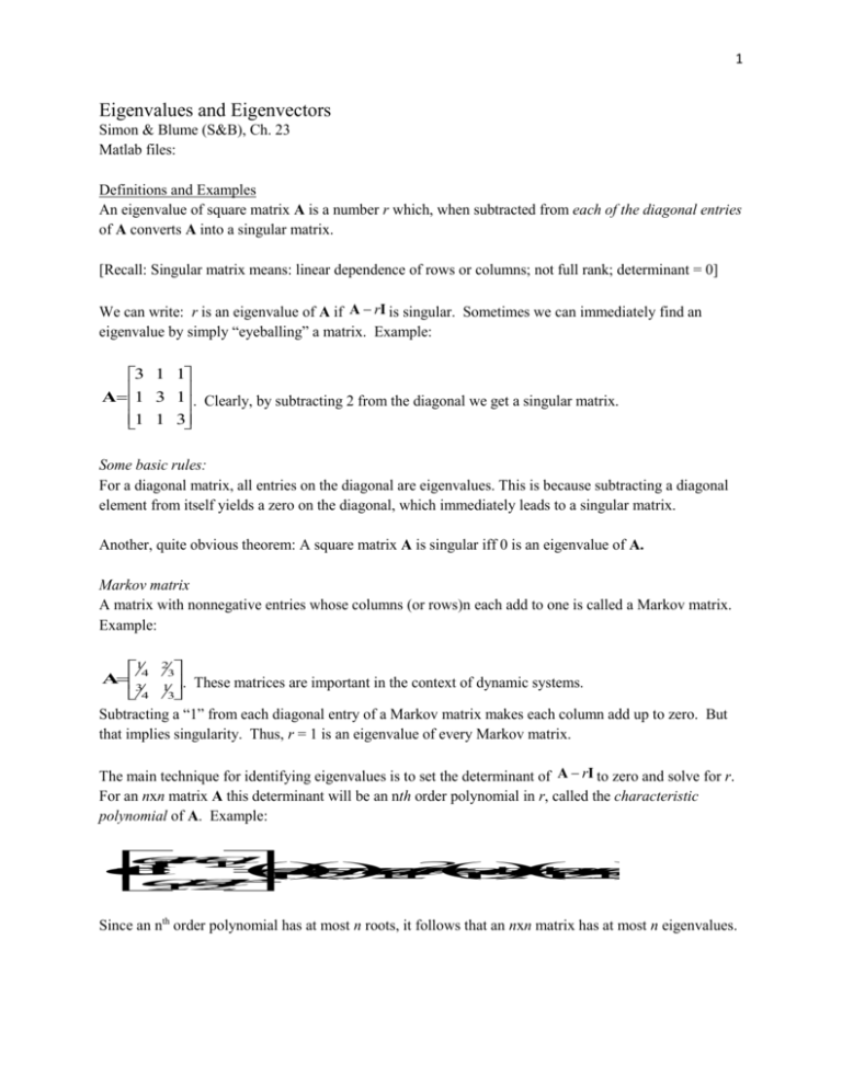
1
Eigenvalues and Eigenvectors
Simon & Blume (S&B), Ch. 23
Matlab files:
Definitions and Examples
An eigenvalue of square matrix A is a number r which, when subtracted from each of the diagonal entries
of A converts A into a singular matrix.
[Recall: Singular matrix means: linear dependence of rows or columns; not full rank; determinant = 0]
We can write: r is an eigenvalue of A if A  rI is singular. Sometimes we can immediately find an
eigenvalue by simply “eyeballing” a matrix. Example:
3 1 1

A 
1 3 1 . Clearly, by subtracting 2 from the diagonal we get a singular matrix.
1 1 3


Some basic rules:
For a diagonal matrix, all entries on the diagonal are eigenvalues. This is because subtracting a diagonal
element from itself yields a zero on the diagonal, which immediately leads to a singular matrix.
Another, quite obvious theorem: A square matrix A is singular iff 0 is an eigenvalue of A.
Markov matrix
A matrix with nonnegative entries whose columns (or rows)n each add to one is called a Markov matrix.
Example:
14 23
A
. These matrices are important in the context of dynamic systems.
3
 4 13
Subtracting a “1” from each diagonal entry of a Markov matrix makes each column add up to zero. But
that implies singularity. Thus, r = 1 is an eigenvalue of every Markov matrix.
The main technique for identifying eigenvalues is to set the determinant of A  rI to zero and solve for r.
For an nxn matrix A this determinant will be an nth order polynomial in r, called the characteristic
polynomial of A. Example:
a

r
a


1
1
1
2
2
d
e
t

a

r
a

r

a
a

r

a

a
r

a
a

a
a






1
12
2
1
2
2
1
1
1
2
21
1
2
2
1
2
2
1


a
a

r
2
1
2
2


Since an nth order polynomial has at most n roots, it follows that an nxn matrix has at most n eigenvalues.
2
Eigenvectors
Recall that a square matrix B is nonsingular iff the only solution of Bx  0 is x  0 . Conversely, B is
singular iff there exists a nonzero x s.t. Bx  0 . Examples:
Not singular:
12


B



01


x


1
x



x
2


x

2
x


1
2
B
x


0

x

0
,x

0
,
1
2
 x 
 2 
Singular:
12


B



24


B

1
x


1
x



x
2



2
x
x
1
2
B
x


0

x

2
,x


1
, B

0
1
2


2
x

4
x
1
2


It follows that if r is an eigenvalue of the square matrix A, the system of equations ArIc0has a
solution other than c  0 .
Such a vector c is called the eigenvector of A corresponding to the eigenvalue r. We can write:
A
c

r
I
c

0 A
cr
c
For examples of finding eigenvalues and eigenvectors see S&B, p. 583. For a given eigenvalue, there
usually exists an infinite set of eigenvectors. They form what’s called the eigenspace of A w.r.t. a given
eigenvalue.
Solving Linear Difference Equations
Eigenvalues and eigenvectors can be useful in solving k-dimensional dynamical problems modeled with
linear difference equations. To warm-up, let’s look at such an equation in k = 1 dimension:
yt 1  ayt
for some constant a. An example would be an interest-accumulating account with yt11yt where
 is the interest rate. A solution to this difference (or dynamic) equation is an expression for yt in terms
of the initial amount y0 , a, and t. In this case, we can find the solution via recursive substitution:
3
y1  ay0
y2  ay1  a 2 y0
yt  at y0
Now consider a system of two linear difference equations with cross-dependence (i.e. the equations are
coupled):
xt1 axt byt
yt1 cxt dyt
In matrix form, this can be written as
x
x
ab




t

1
t
z



A
z
t
+
1
t





y
y
c
d
t

1
t

 

If b = c = 0 the two equations become uncoupled, and can be easily solved:
t
x
a
x
x
a
x
t
1
t
t
0
t
y
d
y
y
a
y
t
1
t
t
0
When the equations are coupled, the system can be solved by first finding a change of variables that
uncouples them. S&B provide a concrete example (p. 588) of this technique. We’ll jump right into the
abstract (i.e. general) case. Consider the following two-dimensional system of difference equations:
zt+1  Azt
Assume there exists a 2x2 non-singular, invertible “change-of-coordinate” matrix C s.t.
z

C
Z
,
1
Z

C
z
and
  
1
1
1
1
1
Z

C
z

C
A
z

C
A
z

C
A
C
Z

C
A
C
Z




t
+
1
t
+
1
t
t
t
t


-1
Now, if C AC were a diagonal matrix the transformed system of difference equations would be
uncoupled and thus easily solved. So the question becomes: What kind of matrix C will lead to a


-1
diagonal C AC ?
4
Partition C into its columns, i.e write C as Cc1 c2, and let the desired diagonal matrix be
generically expressed as
r 0
-1
Λ 1
. Thus, we want C ACΛ, or, equivalently, AC CΛ. We can write this as
0
r

2
r


10
A
c

c

A
c
c

r
cc









1c
2
1c
2
1A
2
1
1r
2
2


0
r

2

A
cc

r
A
c

r
c
1
1
1
2
2
2
Thus, we want r1 and r2 to be the eigenvalues of A, and c1 and c 2 the corresponding eigenvectors.
k-dimensional system
Now let A be a k by k matrix, r1 through rk its eigenvalues, and c1 through ck the corresponding
eigenvectors. Then
r
1
CA
C


0

-1
0
Λ


r
k
Generally, if the above holds, the columns of C must be the eigenvectors of A and the diagonal entries of
Λ must be its eigenvalues. We can also write
ACΛC-1 ,
which is the spectral decomposition of A. (See matrix algebra tutorial notes for more details).
Note: Since there exist an infinite number of eigenvectors for each eigenvalue, it is standard procedure to
normalize each column in C s.t. cc  1 (Matlab’s eig command does this automatically)
Now we have the tools to solve a general linear system of difference equations zt+1  Azt . If the
eigenvalues of A are real and distinct, and if we construct C as a matrix of eigenvectors of A, the linear
change of variables z  CZ transforms the system of difference equations to the uncoupled system
1
Z

A
C
C
ZΛ
t
+
1
tZ
t
which we can easily solve as
5
Z 1 , t   1 r1 t
Z 2 , t   2 r 2t
Z k , t   k r kt
where the  -terms are constants that are implicitly defined by the initial conditions for zj , j 1 k.
Transforming back to the original variables yields
z
Z

 
1
,
t
1
,
t



z
Z
2
,
t
2
,
t



z


C

cc

t
  1 2
 
z
Z
k
,
t
k
,
t

 



t


r
1
1
t
r
t
t
t
2
2


c

r
c

r
c


r
c

k
1
1
2
2
2
k
k
k
 1
t
r


k
k





z
Now all we need to complete the solution is knowledge of the initial vector z
0
1
,
0 z
2
,
0

Then, setting t = 0 in yields


z

c

c

c

cc

0
1
1
2
2
k
k
1 2


z
k
,
0
.
 
 


1
1
 
2
2


c

C
.

k
 
 
k
k


 
Thus, by proper choice of the  terms gives the solution of zt+1  Azt for any z 0 . Thus, is often referred
to as the general solution of zt+1  Azt .
The solution to this system can also be derived via matrix powers (see p. 594-5). If we have
C-1ACΛ, then the t-th power of matrix A can be expressed as
t
r
1

t
A
C

0

0
 -1
C
t
rk
And the solution to the system of difference equations with initial condition z 0 can be expressed as
t

r
1

t
z
A
z
C
t
0

0


0
 -1
C
z
0

t
r
k
6
Stability of equilibria
t
If z 0  0 then the solution of zt+1  Azt is zt  0 t , since A 0  0 for all t. A solution of the system
in which z t is the same constant for all t is called a steady state, equilibrium, or stationary solution of the
difference equation. The question arises as to the stability of the steady state solution zt  0 t . We
declare this solution as asymptotically stable if every solution of zt+1  Azt tends to the steady state
z  0 as t tends to infinity.
Since gives every solution for different values of the  terms, we conclude that every solution tends to
t
zero iff each ri tends to zero. Since the r-terms are eigenvalues of A and since they go to zero only if
r  1 , we can state the following theorem:
If the k by k matrix A has k distinct real eigenvalues, then every solution of the general system of linear
difference equations tends to zero iff all eigenvalues of A satisfy r  1 .