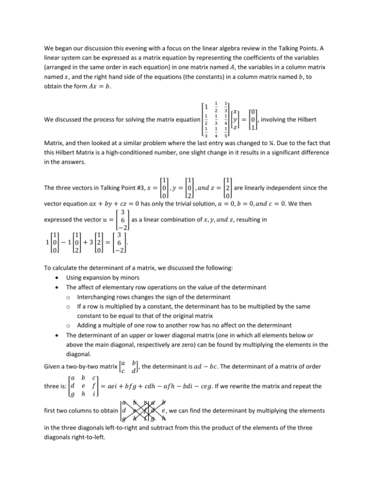
We began our discussion this evening with a focus on the linear algebra review in the Talking Points. A
linear system can be expressed as a matrix equation by representing the coefficients of the variables
(arranged in the same order in each equation) in one matrix named 𝐴, the variables in a column matrix
named 𝑥, and the right hand side of the equations (the constants) in a column matrix named 𝑏, to
obtain the form 𝐴𝑥 = 𝑏.
1
We discussed the process for solving the matrix equation
1
2
1
[3
1
2
1
3
1
4
1
3 𝑥
1
[𝑦]
4
1 𝑧
5]
0
= [0], involving the Hilbert
1
Matrix, and then looked at a similar problem where the last entry was changed to ¼. Due to the fact that
this Hilbert Matrix is a high-conditioned number, one slight change in it results in a significant difference
in the answers.
1
1
1
The three vectors in Talking Point #3, 𝑥 = [0] , 𝑦 = [0] , 𝑎𝑛𝑑 𝑧 = [2] are linearly independent since the
0
2
0
vector equation 𝑎𝑥 + 𝑏𝑦 + 𝑐𝑧 = 0 has only the trivial solution, 𝑎 = 0, 𝑏 = 0, 𝑎𝑛𝑑 𝑐 = 0. We then
3
expressed the vector 𝑢 = [ 6 ] as a linear combination of 𝑥, 𝑦, 𝑎𝑛𝑑 𝑧, resulting in
−2
1
1
1
3
1 [0] − 1 [0] + 3 [2] = [ 6 ].
0
2
0
−2
To calculate the determinant of a matrix, we discussed the following:
 Using expansion by minors
 The affect of elementary row operations on the value of the determinant
o Interchanging rows changes the sign of the determinant
o If a row is multiplied by a constant, the determinant has to be multiplied by the same
constant to be equal to that of the original matrix
o Adding a multiple of one row to another row has no affect on the determinant
 The determinant of an upper or lower diagonal matrix (one in which all elements below or
above the main diagonal, respectively are zero) can be found by multiplying the elements in the
diagonal.
𝑎 𝑏
Given a two-by-two matrix [
], the determinant is 𝑎𝑑 − 𝑏𝑐. The determinant of a matrix of order
𝑐 𝑑
𝑎 𝑏 𝑐
three is: [𝑑 𝑒 𝑓 ] = 𝑎𝑒𝑖 + 𝑏𝑓𝑔 + 𝑐𝑑ℎ − 𝑎𝑓ℎ − 𝑏𝑑𝑖 − 𝑐𝑒𝑔. If we rewrite the matrix and repeat the
𝑔 ℎ 𝑖
𝑎 𝑏 𝑐 𝑎 𝑏
first two columns to obtain |𝑑 𝑒 𝑓 | 𝑑 𝑒 , we can find the determinant by multiplying the elements
𝑔 ℎ 𝑖 𝑔 ℎ
in the three diagonals left-to-right and subtract from this the product of the elements of the three
diagonals right-to-left.
I did not quite understand the discussion on the even and odd permutations. I could follow why the
permutation was considered even or odd, but I did not understand the purpose.
Next, we discussed how to find the inverse of a matrix using row operations. Taking the original matrix,
𝑎 𝑏 𝑐 1 0 0
along-side its corresponding identity matrix, for example,[𝑑 𝑒 𝑓 ⋮ 0 1 0], we convert the matrix
𝑔 ℎ 𝑖 0 0 1
into reduced row-echelon form which means the matrix on the left is now the identity matrix and the
matrix on the right is the inverse. If this cannot be achieved, the matrix is singular.
Our discussion then moved to that of finding the characteristic polynomial and the eigenvalues and
eigenvectors for a given matrix. The characteristic polynomial, 𝑝(𝜆) = det(𝜆𝐼 − 𝐴). Some texts used the
form (𝐴 − 𝜆𝐼) which implies ±𝜆𝑛 .
1 2
For the matrix 𝐴 = [
]:
4 3
𝜆𝐼 − 𝐴
1 2
𝜆 0
𝜆 − 1 −2
[
]−[
]=[
]
4 3
𝜆 0
−4 𝜆 − 3
𝜆 − 1 −2
]
−4 𝜆 − 3
𝑝(𝜆) = (𝜆 − 1)(𝜆 − 3) − 8
𝑝(𝜆) = 𝜆2 − 4𝜆 − 5
And the eigenvalues are 𝜆 = 5 𝑎𝑛𝑑 𝜆.
𝑥
1 2 𝑥
The eigenvector for 𝜆 = 5: [
] [ ] = 5 [𝑦] yields the equations
4 3 𝑦
𝑥 + 2𝑦 = 5𝑥 and
4𝑥 + 3𝑦 = 𝑦
1
Solving, we find that 𝑦 = 2𝑥; therefore the eigenvector is [ ]. Using the same method, we find the
2
1
eigenvector for 𝜆 = −1 is [ ].
−1
𝑝(𝜆) = 𝑑𝑒𝑡 [
The eigenvalues for a matrix that is upper or lower diagonal come from the diagonal. For the upper
1 1 1 1
𝜆−1
1
1
1
0 1 1 1
0
𝜆
−
1
1
1
diagonal matrix 𝐶 = [
], where (𝜆𝐼 − 𝐴) = [
], the
0 0 1 1
0
0
𝜆−1
1
0 0 0 1
0
0
0
𝜆−1
4
determinant is (𝜆 − 1) , which yields the eigenvalue 𝜆 = 1.
0 2 1
To find the eigenvalues for the matrix 𝐴 = [1 0 0], we found that the characteristic polynomial
0 1 0
3
𝑝(𝜆) = 𝜆 − 2𝜆 − 1 could not be factored. We discussed using either synthetic division or long division
to solve. Two of the eigenvalues looked VERY familiar, 𝜆 =
1+√5
2
1
= 𝜌 and 𝜆 = 1 − 𝜌 = − 𝜌, and the
third 𝜆 = −1.
1 1
To return to the Fibonacci studies we looked at matrix 𝐴 = [
].
1 0
𝐹
For 𝑥⃗0 = [ 1 ],
𝐹0
𝑥⃗𝑛+1 = 𝐴𝑥⃗𝑛
𝑥⃗𝑛 = 𝐴𝑛 𝑥⃗0
Theorem: if 𝜆1 , 𝜆2 , … 𝜆𝑚 are mutually distinct eigenvalues of A with eigenvectors 𝑥⃗1 , 𝑥⃗2 , … 𝑥⃗𝑚 , then
{𝑥⃗1 , 𝑥⃗2 , … 𝑥⃗𝑚 , } is a linearly independent set.
The Power Method showed us that an n x n matrix A with eigenvalues 𝜆1 , 𝜆2 , … 𝜆𝑚 and eigenvectors
𝑥⃗1 , 𝑥⃗2 , … 𝑥⃗𝑚 that are linearly independent, if we assume that |𝜆1 | > |𝜆2 | ≥ |𝜆3 | ≥ ⋯ , 𝜆1 is the
dominant eigenvalue. To prove this we began with a vector x that was a linear combination of
eigenvectors. Then, 𝐴𝑥⃗ = 𝐴(𝑐1 𝑥⃗1 + 𝑐2 𝑥⃗2 + … 𝑐𝑛 𝑥⃗𝑛)
= 𝑐1 𝐴𝑥⃗1 + 𝑐2 𝐴𝑥⃗2 + … 𝑐𝑛 𝐴𝑥⃗𝑛
= 𝑐1 𝜆1 𝑥⃗1 + 𝑐2 𝜆2 𝑥⃗2 + … 𝑐𝑛 𝜆𝑛 𝑥⃗𝑛
2
𝐴 𝑥⃗ = 𝑐1 𝜆21 𝑥⃗1 + 𝑐2 𝜆2 2 𝑥⃗2 + … 𝑐𝑛 𝜆2 𝑛 𝑥⃗𝑛
𝐴𝑘 𝑥⃗ = 𝑐1 𝜆𝑘 1 𝑥⃗1 + 𝑐2 𝜆𝑘 2 𝑥⃗2 + … 𝑐𝑛 𝜆𝑘 𝑛 𝑥⃗𝑛
1 𝑘
𝜆2 𝑘
𝜆𝑛 𝑘
𝐴
𝑥
⃗
=
𝑐
𝑥
⃗
+
𝑐
(
)
𝑥
⃗
+
…
𝑐
(
) 𝑥⃗
1 1
2
2
𝑛
𝜆𝑘 1
𝜆1
𝜆1 𝑛 𝑛
lim
1
𝑘→∞ 𝜆𝑘 1
𝐴𝑘 𝑥 = 𝑐1 𝑥⃗1
After normalization, 𝐴𝑘 𝑥⃗ converges to an eigenvector of A associated with the dominant eigenvalue.
𝐹
1 1 𝐹𝑛+1
In the Fibonacci case where 𝐴 = [
], [
] = 𝐴𝑛 [ 1 ]. Factoring, we have
𝐹0
𝐹𝑛
1 0
𝐹𝑛+1
𝑟
𝐹
𝐹𝑛 , [ 𝐹𝑛 ] = 𝐹 𝑛 [ 𝑛 ] = 𝐴𝑛 [ 1 ], where 𝑟 𝑛 is the ratio of consecutive terms.
𝐹0
1
1
The characteristic polynomial is 𝑝𝜆) = 𝜆2 − 𝜆 − 1, where the dominant eigenvalue is 𝜆 = 𝜌 𝑜𝑟 1.618 …
1
and the other eigenvalue is 𝜆 = − 𝜌 𝑜𝑟 − .618.
The discussion then turned to that of Discrete Population Models. In this model, rabbits die and are
therefore taken out of the reproductive cycle after three births. Using an Excel spreadsheet we were
able to find the growth ratio and the fixed growth rate of this model. The growth ratio approached a
value of 1.465555, or a rate of 46%. This remained true even when we changed the initial populations.
While I understood this part of the discussion, I have been unable to recreate it in Excel because I was
not able to create a spreadsheet myself during the lecture and while trying to follow the steps did not
have time to write down the formula used to generate the cells for the 𝑥1 , 𝑥2 , 𝑎𝑛𝑑 𝑥3 columns. I hope
that we will continue with this model so that I can gain a better understanding of how the successive
generations of rabbits are found.