STAT 6305 — Unit 5: How a Block Design Differs From a One-Way ANOVA— Partial Solutions
5.1.1.
[Enter and print out data.]
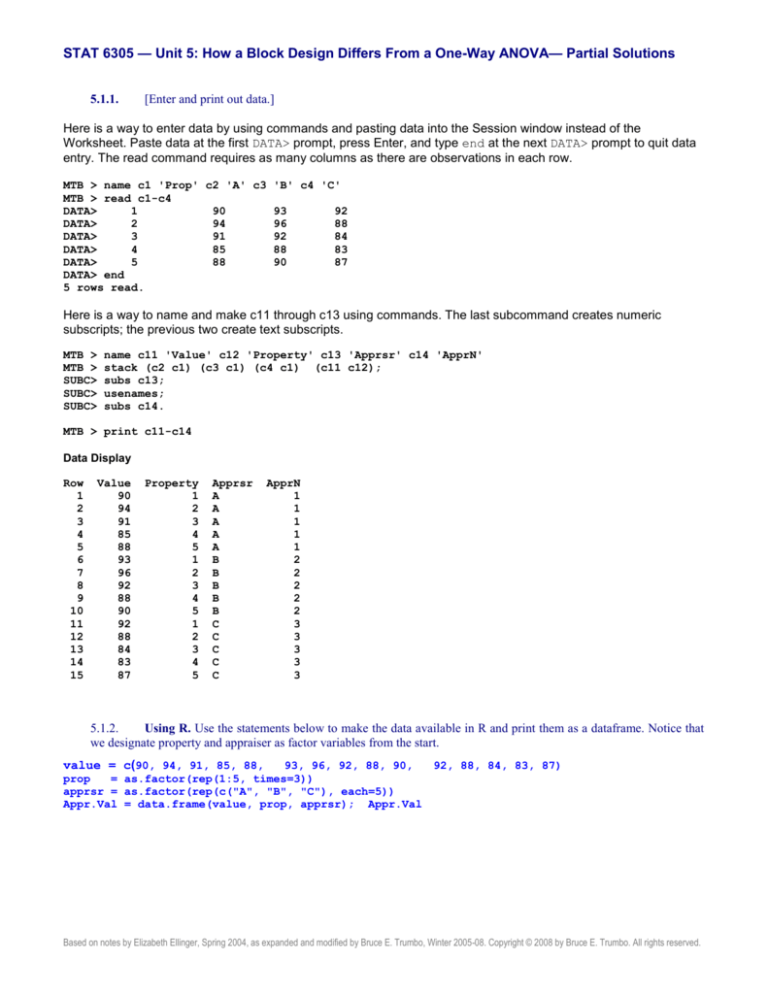
Here is a way to enter data by using commands and pasting data into the Session window instead of the
Worksheet. Paste data at the first DATA> prompt, press Enter, and type end at the next DATA> prompt to quit data
entry. The read command requires as many columns as there are observations in each row.
MTB > name c1 'Prop' c2 'A' c3 'B' c4 'C'
MTB > read c1-c4
DATA>
1
90
93
92
DATA>
2
94
96
88
DATA>
3
91
92
84
DATA>
4
85
88
83
DATA>
5
88
90
87
DATA> end
5 rows read.
Here is a way to name and make c11 through c13 using commands. The last subcommand creates numeric
subscripts; the previous two create text subscripts.
MTB >
MTB >
SUBC>
SUBC>
SUBC>
name c11 'Value' c12 'Property' c13 'Apprsr' c14 'ApprN'
stack (c2 c1) (c3 c1) (c4 c1) (c11 c12);
subs c13;
usenames;
subs c14.
MTB > print c11-c14
Data Display
Row
1
2
3
4
5
6
7
8
9
10
11
12
13
14
15
Value
90
94
91
85
88
93
96
92
88
90
92
88
84
83
87
Property
1
2
3
4
5
1
2
3
4
5
1
2
3
4
5
Apprsr
A
A
A
A
A
B
B
B
B
B
C
C
C
C
C
ApprN
1
1
1
1
1
2
2
2
2
2
3
3
3
3
3
5.1.2.
Using R. Use the statements below to make the data available in R and print them as a dataframe. Notice that
we designate property and appraiser as factor variables from the start.
value = c(90, 94, 91, 85, 88,
93, 96, 92, 88, 90,
92, 88, 84, 83, 87)
prop
= as.factor(rep(1:5, times=3))
apprsr = as.factor(rep(c("A", "B", "C"), each=5))
Appr.Val = data.frame(value, prop, apprsr); Appr.Val
Based on notes by Elizabeth Ellinger, Spring 2004, as expanded and modified by Bruce E. Trumbo, Winter 2005-08. Copyright © 2008 by Bruce E. Trumbo. All rights reserved.
Stat 6305 — Unit 5: Partial Solutions
2
> Appr.Val = data.frame(value, prop, apprsr);
value prop apprsr
1
90
1
A
2
94
2
A
3
91
3
A
4
85
4
A
5
88
5
A
6
93
1
B
7
96
2
B
8
92
3
B
9
88
4
B
10
90
5
B
11
92
1
C
12
88
2
C
13
84
3
C
14
83
4
C
15
87
5
C
Appr.Val
5.2.1.
Find the means for each appraiser with the command table c13; subcommand means c11. or with the command
describe c11; subcommand by c13.).
MTB > table c13;
SUBC> means c11.
Tabulated statistics: Apprsr
Rows: Apprsr
Value
Mean
A
B
C
All
89.60
91.80
86.80
89.40
MTB > desc c11;
SUBC> by c13;
SUBC> mean.
Descriptive Statistics: Value
Variable
Value
Apprsr
A
B
C
Mean
89.60
91.80
86.80
5.2.2.
Make a standard graphics plot of Value against Property, with points labeled to indicate Appraisers. What are
the advantages and disadvantages of the pixel graphics plot compared with the character graphics plot?... Describe the
results of the command lplot c11 c14 c12.
The subcommands make a more readable x-axis.
MTB >
MTB >
SUBC>
SUBC>
gstd
lplot c11 c12 c14;
xstart 1;
xincr 1.
Page 2 of 13
Stat 6305 — Unit 5: Partial Solutions
3
Character Letter Plot
B
95.0+
A
Value
- B
- C
B
A
90.0+ A
B
C
B
A
C
85.0+
A
C
C
+---------+---------+---------+---------+Property
1.0
2.0
3.0
4.0
5.0
The pixel graphics plot is more attractive, easier to read (in most cases), and can use either text or numeric data to
designate categories (levels of a factor). The standard graphics plot requires less storage and so makes for reports
with shorter file lengths.
Notice that, for four of the five properties, Appraiser C gave the lowest value.The command lplot c11 c13 c12
results in the character graph below. We used subcommands to control the x-axis.
MTB > lplot c11 c14 c12;
SUBC> xstart 1;
SUBC> xincr 1.
Character Letter Plot
95.0+
Value
90.0+
85.0+
-
B
B
A
C
C
A
E
E
D
A
B
E
D
C
D
+---------+---------+ApprN
1.0
2.0
3.0
By switching the position of c12 and c14 in the command, the x-axis becomes appraiser instead of property. Thus,
this graph illustrates Value against Appraiser by Property. Here the five properties are designated by letters A-E
(instead of using 1-5). Appraisers, on the x-axis are designated 1, 2, and 3 (instead of A, B, and C). Again here, we
see the tendency of Appraiser C to give the lowest values.
Page 3 of 13
Stat 6305 — Unit 5: Partial Solutions
4
Finally, we show a pixel graph of Value against Appraiser (numeric coding), with colored symbols to designate
Properties.
Scatterplot of Value vs ApprN
Property
1
2
3
4
5
96
94
Value
92
90
88
86
84
82
1.0
1.5
2.0
ApprN
2.5
3.0
At this point it is appropriate for you to consider, if you were writing a report with room for only one graphic display
of the data, whether you would designate Appraisers or Properties by symbols. What is the message you want to
communicate, and which graphic tells your story best? (There is no "right" answer, but personal preferences are
allowed!)
5.2.3.
Using R. Use the R code below (one block at a time) to make three graphical displays of the data. The first
two are also exercises in data types, so explain their use. The interaction plot is intended for use with slightly more
advanced designs but serves well here with appropriate labeling; it is programmed to handle factor variables directly.
colr = c("red", "blue", "darkgreen")
plot(as.numeric(prop), value, pch=as.character(apprsr), col=colr[as.numeric(apprsr)],
xlab="Property", ylab="Value", main="Appraised Values by Property and Appraiser")
Page 4 of 13
Stat 6305 — Unit 5: Partial Solutions
5
plot(0, xlim=c(1,5), ylim=c(80,100), type="n", xlab="Property", ylab="Value",
main="Appraised Values by Property and Appraiser") # set up but no plot
char = unique(apprsr)
for (i in 1:3) {
lines(value[as.numeric(apprsr)==i], type="b", col=colr[i],
pch=as.character(unique(apprsr))[i]) } # no x-variable given, indices 1:5 used
as x
Variables prop and apprsr are defined as factor variables. In order to use them as numeric and character
variables, functions to change variable type are required.
interaction.plot(prop, apprsr, value, xlab="Property", ylab="Value",
main="Appraised Values by Property and Appraiser")
Page 5 of 13
Stat 6305 — Unit 5: Partial Solutions
6
5.2.4. Using R. Display three boxplots using plot(apprsr, value) and also using
boxplot(value ~ apprsr). What do you get with plot(as.numeric(apprsr), value)?
> plot(apprsr, value)
boxplot(value ~ apprsr)
Same plot as above.
plot(as.numeric(apprsr), value, pch=19)
Page 6 of 13
Stat 6305 — Unit 5: Partial Solutions
7
5.3.1.
Make a normal probability plot of the residuals from this ANOVA model. Does it show that the data are
reasonably close to normal? Perform an appropriate test of normality and give the P-value.
The probability plot of the residuals calculated from the ANOVA on p. 5-4 of Unit 5 is as follows:
Probability Plot of Residuals
Normal - 95% CI
99
Mean
StDev
N
AD
P-Value
95
90
9.473903E-15
1.509
15
0.163
0.929
Percent
80
70
60
50
40
30
20
10
5
1
-5.0
-2.5
0.0
Residuals
2.5
5.0
The points are very close to a straight line and well within the confidence bands. The high P-value of .929 indicates
that the null hypothesis of normality cannot be rejected for these data.
Note: If the P-value for a goodness-of-fit test is above 95%, and certainly if it is above 99% (this one is about 93%),
one is entitled to wonder if the fit is "too good to be true." For example, fit that is a lot better than one would expect
considering typical random variation may indicate fake data.
5.3.2.
Compare the test for the Appraiser effect with the test for the Property effect. How is it possible that the two
P-values are nearly equal when the F-statistics have quite different values (7.88 vs. 6.33)?
The shape of an F distribution is determined by its two degrees-of-freedom parameters (the numerator and
denominator df). These parameters affect the shape of an F-distribution. The Appraiser and the Property effects
have different degrees of freedom. Thus, their F-distributions under their respective null hypotheses will be
different. Here it happens that the area to the right of 7.88 under one F-distribution density curve is about the same
as the area to the right of 6.33 under a different density curve.
5.3.3.
Explain in plain English what it would mean about the values of properties if the Property effect was not found
to be significant.
If the Property effect was not found to be significant, it might mean that the properties were similar enough that the
same appraiser would tend appraise them all at approximately the same value. (Perhaps all of the properties were in
the same tract.) Another possibility would be that properties in the population have quite variable values, but that our
sample is too small to detect the variation. (That is, test of the null hypothesis for Properties may have poor power.)
5.3.4.
“Consider the variance components in Minitab's EMS table. The variance component for Error is the estimated
value of σ2, which we have already seen to be MS(Err) = 3.983. The variance component for Property is the estimated
value of σB2. But MS(Prp) estimates σ2 + 3σB2, not σB2. How can the values of MS(Prp) and MS(Err) be used together to
obtain a numerical estimate of σB2? Show that your answer agrees with the variance component for Property shown in the
EMS table.”
To estimate σB2, use the following equation:
Estimate of σB2 = (MS(Prp) – MS(Err))/3 = (25.233 – 3.983)/3 = 7.083
This value is in agreement with the variance component of 7.083 shown in the EMS table of Section 5.3.
Page 7 of 13
Stat 6305 — Unit 5: Partial Solutions
8
5.3.5.
“If you own 5 similar properties, consider selling them, and wonder if they should all be put on the market at
the same price, you might consult three appraisers (randomly chosen from among the many available) for advice. In this
case, how would the ANOVA model be changed?”
In this case, Property () would be a fixed effect. You are not picking the properties at random, you are
investigating properties you own. Also, Appraiser (A) would be a random effect. The model would become
Yij = + Ai + j + eij, where i = 1, 2, 3; j = 1, ..., 5; i i = 0; Aj iid N(0, A2); and eij iid N(0, 2). In this case the
Appraisers play the role of blocks and the Properties are the main effect under investigation. [This is similar to the
situation in an earlier unit where garages (appraisers) said how much it would cost to repair a car (buy a property).]
The lesson here is that you have to pay close attention to the story behind the data in order to know the correct
method of analysis. Just looking at the data in a table is not enough.
5.3.6.
... The relative efficiency of a block design compared to a one-way ANOVA is defined as the ratio
RE = MS(Err)OneWay/MS(Err)Block. The block design uses bt observations. The idea is that a one-way ANOVA would
require about bt(RE) total observations to do the "same job." ... [E]stimate MS(Err)OneWay from the ANOVA table of the
block experiment as MS(Err)OneWay [(b – 1)MS(Block) + b(t – 1)MS(Error)] / (bt – 1). In our data b = 5 and t = 3. Find
RE for these data. How many observations (instead of b = 5) on each of t = 3 Appraisers does your value of RE indicate
we would need for a one-way ANOVA having a "precision" equivalent to our blocked experiment?
For our data MS(Block) = MS(Property) = 25.233 and MS(Error) = 3.983. Thus the estimate of MS(Error) OneWay is
[4(25.233) + 10(3.983)] / 14 = 10.054 and the estimated RE is 10.054 /3.983 = 2.52. The required total sample size
for such a 3-treatment one-way design is 15(2.52) randomly chosen properties. This means that each of the three
Appraisers would have to assess 5(2.52) or about 13 randomly assigned properties (the convention is to round up).
Not only would each Appraiser have to do more work, but also we would need to sample a total of 39 properties
(compared with 5 in the block design). The above formula for RE is given on p955 of O/L 6e.
5.4.1.
Perform an INCORRECT one-way ANOVA using Property as the factor. Compare the results with the correct
ANOVA table from the block design.
This INCORRECT procedure gives the following output:
MTB > onew 'Value' 'Property'
One-way ANOVA: Value versus Property
Source
Property
Error
Total
S = 3.077
Level
1
2
3
4
5
N
3
3
3
3
3
DF
4
10
14
SS
100.93
94.67
195.60
MS
25.23
9.47
R-Sq = 51.60%
Mean
91.667
92.667
89.000
85.333
88.333
StDev
1.528
4.163
4.359
2.517
1.528
F
2.67
P
0.095
R-Sq(adj) = 32.24%
Individual 95% CIs For Mean Based on
Pooled StDev
-------+---------+---------+---------+-(---------*---------)
(---------*---------)
(---------*--------)
(---------*---------)
(---------*---------)
-------+---------+---------+---------+-84.0
88.0
92.0
96.0
The correct block design yields a P-value of .013 for Property (significant effect at the 5% level), but the incorrect
one-way ANOVA yields a P-value of .095 (not significant). In the one-way ANOVA, SS(Error) = 94.67, which is
much larger than SS(Error) = 31.867 in the randomized block design. This is due to the fact that SS(Appraiser) =
62.80 is separated out from SS(Error) in the block design, but not in the one-way ANOVA.
Page 8 of 13
Stat 6305 — Unit 5: Partial Solutions
9
5.4.2.
Suppose you were trying to analyze data from a block design using the limited capabilities of a spread sheet, in
which the one-way ANOVA is the only ANOVA procedure available. How could you use output from the spreadsheet to
put together the correct analysis?
The one way ANOVA could be run twice: once for Appraiser as the treatment and once for Property as the
treatment. The SS(Appraiser) term calculated in the first run and the SS(Property) term calculated in the second
run would be correct and SS(Total) would be the same for both runs. Then the correct value of SS(Error) for the
block ANOVA could be found by subtraction: SS(Error) = SS(Total) – [SS(Appr) + SS(Prop)].
5.5.1.
[New Data] Put the component lifetime data into a Minitab worksheet. (a) Then use Minitab's ability to do
cross-tabulations to obtain a table of the data suitable for presentation to human readers, similar to the first table shown
above. (Command table 'Temp' 'Batch'; with subcommand data 'Months'.)
MTB > table 'Temp' 'Batch';
SUBC> data 'Months'.
Tabulated statistics: Temp, Batch
Rows: Temp
Columns: Batch
1
2
3
4
5
1
3.35
4.91
3.07
15.26
5.09
2
6.33
1.06
1.78
24.11
10.19
3
0.53
0.91
1.45
1.79
5.16
Cell Contents:
Months
:
DATA
5.5.2.
Make a labeled scatterplot of the original lifetime data similar to the one for the appraiser data in
Section 4.2. Perform an ANOVA for a block design on the original lifetimes. Make a plot of residuals against fits.
Interpret the results.
MTB > Plot 'Months'*'Batch';
SUBC>
Symbol 'Temp'.
Scatterplot of Months vs Batch
25
Temp
1
2
3
Months
20
15
10
5
0
1
2
3
Batch
4
5
Notice that the highest Temperature level (coded 3) tends to have the shortest lifetimes in each Batch. This is a
preliminary indication that there may be a significant Temperature effect. However, within Batch variability may not
be consistent. ANOVA procedures do not work well under heteroscedasticity, so the effect (if real) may be masked.
MTB > Name c14 "RESI1"
MTB > ANOVA 'Months' = Temp Batch;
SUBC>
Random 'Batch';
Page 9 of 13
Stat 6305 — Unit 5: Partial Solutions
SUBC>
10
Residuals 'RESI1'.
ANOVA: Months versus Temp, Batch
Factor
Temp
Batch
Type
fixed
random
Levels
3
5
Values
1, 2, 3
1, 2, 3, 4, 5
Analysis of Variance for Months
Source
Temp
Batch
Error
Total
DF
2
4
8
14
SS
116.46
286.18
181.86
584.51
S = 4.76788
MS
58.23
71.55
22.73
F
2.56
3.15
R-Sq = 68.89%
P
0.138
0.079
R-Sq(adj) = 45.55%
In contrast to the ANOVA on the log-transformed data shown in Section 5.5, this ANOVA on the original data shows
no significant effects.
Residuals Versus the Fitted Values
(response is Months)
Residual
5
0
-5
-10
0
4
8
Fitted Value
12
16
There are 15 cells (Temperature by Batch combinations) in the data table. Thus there are 15 fitted values on the
horizontal axis. The residuals show a strong tendency to increase in magnitude (absolute value) as the fitted value
increases. This tendency towards heteroscedasticity may be the reason we detected no significant effects for the
untransformed data.
5.5.3.
The ANOVA for the block design on the log-transformed data is shown in this section. Perform it for yourself,
making a normal probability plot of the residuals. Does this plot seem more nearly linear than the one shown in this
section for the original data? Make a plot of residuals against fits and compare it with the one in the previous problem.
Finally, did transforming the data change your interpretation of the data (as to significant differences among the
Temperatures)? How would you report your findings?
We do not repeat the ANOVA table here, but recall that it shows a significant Temperature effect (P-value = 4.1%).
Below we show first the plot of residuals against fits for the transformed data, noting that it shows no pattern of
heteroscedasticity.
Instead of the normal probability plot that can be generated as an option in Minitab's balanced ANOVA procedure,
we show the version with confidence bands provided in the menu path GRAPH Probability plot Single,
normal. The residuals of the transformed data do not fit a normal distribution any better than did the residuals of the
original data.(if anything, maybe worse).
Page 10 of 13
Stat 6305 — Unit 5: Partial Solutions
11
The purpose of transformation is not to make the data normal. It is to try to cure the damaging consequences of
nonnormal data: heteroscedasticity. The plot of residuals against fitted values indicates we have succeeded in that.
Residuals Versus the Fitted Values
(response is LogMo)
0.50
Residual
0.25
0.00
-0.25
-0.50
-0.75
-1.00
0.0
0.5
1.0
1.5
Fitted Value
2.0
2.5
3.0
Normal Probability Plot of Residuals for Log-Transformed Lifetimes
Normal - 95% CI
99
Mean
StDev
N
AD
P-Value
95
90
-8.14164E-17
0.5534
15
0.602
0.096
Percent
80
70
60
50
40
30
20
10
5
1
MTB >
SUBC>
SUBC>
SUBC>
-2
-1
0
RESI3
1
2
desc 'LogMo' 'Months';
by 'Temp';
means;
medians.
Descriptive Statistics: LogMo, Months
Variable
LogMo
Temp
1
2
3
Mean
1.655
1.597
0.373
Median
1.591
1.845
0.372
Months
1
2
3
6.34
8.69
1.968
4.91
6.33
1.450
Page 11 of 13
Stat 6305 — Unit 5: Partial Solutions
12
Based on the log-transformed data, we can report that Temperature makes a difference in the length of life of these
components. In particular, it seems clear that the shortest lifetimes (about 2 months on average for the five Batches
tested) were for components tested at the highest of the three Temperatures. Components tested at lower
temperatures survived for more than 6 months on average. But explicit multiple comparisons (differences among
group means) need to be made with care because of the log transformation. See the next problem.
5.5.4. Perform Fisher's LSD and Tukey's HSD by hand. Use the transformed data. However, notice that a difference in
logarithms (as in these multiple comparisons) is the logarithm of a ratio. How can you use this fact to compare lifetimes
in months (original data scale) for different Temperatures. Use the LSD and HSD formulas in your text for the oneway ANOVA, except that the appropriate variance estimate is the MS(Err) for the block design. (The exact formula for
Fisher's LSD is found in O/L 6e, page 1140; use the formula for "no missing data.") Verify your results for Tukey's HSD
by using Minitab's glm procedure:
LSD = t* [MS(Error) (2/b)]1/2 = 2.306[0.5359 (2/5)]1/2 = 1.068, where t* = 2.306 is the value that cuts off 2.5% from
the upper tail of the t distribution with df = 8. The smallest absolute difference between sample means of logtransformed values is |1.655 – 1.597| = 0.058 < LSD, and so not significant. The next smallest absolute difference
is |1.597 – 0.373| = 1.224 > LSD, and so significant. The underline diagram, in terms of degrees Celsius is
20 35 50. In terms of lifetimes x in months (untransformed data) a difference ln(x1) – ln(x2) = ln(x1/x2) > 1.068 is
significant, and so the ratio x1/x2 > exp(1.068) = 2.91 is significant on the original scale. Roughly speaking, one
mean lifetime (in months) has to be about three times as large as another to be significant. These comparisons are
at the 5% level in the sense that there is a 5% chance of incorrectly declaring any one difference to be significant.
(We know of no way to perform in Minitab the correct Fisher LSD comparisons for levels of the main factor in a
block design.)
In this case, because of the log transformation, "mean" refers to the geometric mean (nth root of the product of n
observations). In the output for the previous problem, notice that the arithmetic ("ordinary") mean lifetime 8.69
months for 33C exceeds the arithmetic mean lifetime 6.34 months for 20C, whereas the geometric mean lifetime
exp(1.655) = 5.23 months for 20C exceeds the geometric mean lifetime exp(1.597) = 4.94 months for 30C. For
data from the right-skewed exponential distribution, the geometric mean or the median may be a more appropriate
measure of location than the arithmetic mean. Of course, the three group medians for transformed and original data
are in the same order because ln is a monotone increasing transformation.
HSD = W = q*[MS(Error)/b]1/2 = 4.04[0.5359 / 5]1/2 = 1.323, where q* = 4.04 is the value that cuts off 2.5% from
the upper tail of the Studentized range distribution for 3 levels and df = 8. Here even the largest absolute difference
|1.655 – 0.373| = 1.282 < 1.323 does not quite reach significance. In this instance, Tukey's procedure is slightly too
conservative to be useful. (In practice, because the main ANOVA declares that there is a significant difference, the
largest difference would be taken as significant, even if Tukey's procedure is used for multiple comparisons and
fails to declare it significant.) Below is Minitab's version of Tukey's HSD procedure (tests and CIs). These
comparisons using HSD are at the 5% level in the sense that there is a 5% chance that any one of the family of
three differences considered "simultaneously" may be incorrectly declared significant.
MTB > GLM 'LogMo' = Temp Batch;
SUBC>
Random 'Batch';
SUBC>
Brief 2 ;
SUBC>
Pairwise Temp;
SUBC>
Tukey.
General Linear Model: LogMo versus Temp, Batch
Factor
Temp
Batch
Type
fixed
random
Levels
3
5
Values
1, 2, 3
1, 2, 3, 4, 5
Analysis of Variance for LogMo, using Adjusted SS for Tests
Source
Temp
Batch
Error
Total
DF
2
4
8
14
S = 0.732062
Seq SS
5.2398
6.7414
4.2873
16.2685
Adj SS
5.2398
6.7414
4.2873
R-Sq = 73.65%
Adj MS
2.6199
1.6854
0.5359
F
4.89
3.14
P
0.041
0.079
R-Sq(adj) = 53.88%
Page 12 of 13
Stat 6305 — Unit 5: Partial Solutions
13
Tukey 95.0% Simultaneous Confidence Intervals
Response Variable LogMo
All Pairwise Comparisons among Levels of Temp
Temp = 1
Temp
2
3
Lower
-1.381
-2.604
Temp = 2
Temp
3
subtracted from:
Center
-0.058
-1.282
Upper
1.26461
0.04087
--+---------+---------+---------+---(-----------*----------)
(----------*----------)
--+---------+---------+---------+----2.4
-1.2
0.0
1.2
subtracted from:
Lower
-2.546
Center
-1.224
Upper
0.09891
--+---------+---------+---------+---(----------*----------)
--+---------+---------+---------+----2.4
-1.2
0.0
1.2
Tukey Simultaneous Tests
Response Variable LogMo
All Pairwise Comparisons among Levels of Temp
Temp = 1
Temp
2
3
Difference
of Means
-0.058
-1.282
Temp = 2
Temp
3
subtracted from:
SE of
Difference
0.4630
0.4630
T-Value
-0.125
-2.768
Adjusted
P-Value
0.9914
0.0570
T-Value
-2.643
Adjusted
P-Value
0.0685
subtracted from:
Difference
of Means
-1.224
SE of
Difference
0.4630
Again here, no significant differences are found. In the Minitab output, all three CIs cover 0, although the CI for
the difference between Temperature 1 (20C) and Temperature 3 (50C) only barely covers 0.
Note: This very small dataset is from a pilot study preceding a much larger proprietary study. From the more
extensive test data of these devices at these three temperatures, it is known that the three population means all
differ, that shorter lifetimes are associated with higher temperatures, and that batch-to-batch variability is small
enough to be negligible for practical purposes. At the usual operating temperature of 35C, the true mean lifetime
is about 5 months. The true lifetime distribution is probably not exactly exponential (perhaps having a slightly
increasing hazard rate—used not quite "as good as new"), but is certainly closer to exponential than normal. Some
details not affecting the analysis or its interpretation have been changed to preserve confidentiality.
5.5.5.
What are the results of an ANOVA according to a block design on the original (untransformed) data?
What would you say about significance in a report of the analysis of this experiment?
Although reliability data are often more nearly distributed as exponential rather than normal, a normal probability
plot on the residuals from a block ANOVA (temperatures fixed, batches random) of data in this experiment is
consistent with normality. The ANOVA shows no significant difference among temperature group means.
For exponential data a log transformation is often used. A block ANOVA based on the transformed data suggests
a significant temperature effect (4% level), but Tukey's HSD only barely detects a difference between . In contrast,
the less conservative Fisher HSD criterion shows a significant difference between the middle and highest
temperatures. Roughly speaking, the change in lifetimes between groups must be in a 3:1 ratio to achieve
significance in this experiment. Thus there seems to be weak evidence of a temperature effect based on the
current experiment over the 20oC to 50oC temperature range. For best reliability it seems prudent to recommend
use of this component in the 20-35oC temperature range. If use at higher temperatures is contemplated, perhaps a
warning of decreased time to failure at higher temperatures should be given.
Page 13 of 13
