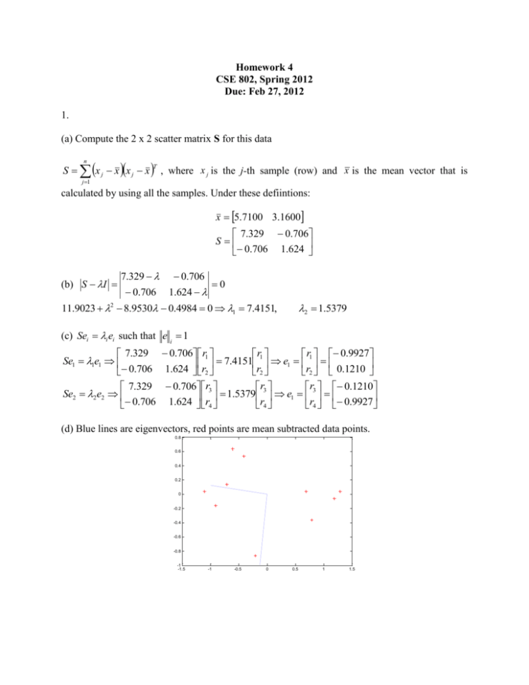
Homework 4
CSE 802, Spring 2012
Due: Feb 27, 2012
1.
(a) Compute the 2 x 2 scatter matrix S for this data
T
S   x j  x x j  x  , where x j is the j-th sample (row) and x is the mean vector that is
n
j 1
calculated by using all the samples. Under these defiintions:
x  5.7100 3.1600
 7.329  0.706
S

 0.706 1.624 
(b) S  I 
7.329  
 0.706
 0.706
1.624  
0
11.9023  2  8.9530  0.4984  0  1  7.4151,
2  1.5379
(c) Sei  i ei such that e i  1
r 
 r   0.9927
 7.329  0.706  r1 
Se1  1e1  
 7.4151 1   e1   1   




 0.706 1.624  r2 
r2 
r2   0.1210 
r 
r   0.1210
 7.329  0.706 r3 
Se2  2e2  
 1.5379 3   e1   3   




 0.706 1.624  r4 
r4 
r4   0.9927
(d) Blue lines are eigenvectors, red points are mean subtracted data points.
0.8
0.6
0.4
0.2
0
-0.2
-0.4
-0.6
-0.8
-1
-1.5
-1
-0.5
0
0.5
1
1.5
2. (a) Since each pattern class has a multivariate Gaussian density with unknown mean vector and
a common but unknown covariance matrix, we will estimate the mean for each class as the mean
of the training patterns for that class.
The way to compute the common covariance matrix is to first compute the covariance matrix of
the three different classes and then average them as the common covariance matrix. The
performance of the plug-in classifier for this data gives the average error rate for 15 rounds cross
validation: 0.0248 and variance of error rate: 0.00051995. The result of individual run is listed in
Table 1.
(b) Since each of the classes has different class mean and covariance matrix, we separate data of
different classes and compute the parameters for each of the pattern class. Also, because their
covariance matrices are different, the resulting decision boundary is quadratic. The average error
rate for these 15 rounds cross validation is: 0.0353. The variance of error rate is: 0.00061515. The
result of individual run is listed in Table 1.
(c) For parzon window classifier:
Window size = 0.01,
Average error rate = 0.6549.
Variance of error rate = 0.0001.
Window size = 0.5,
Average error rate is 0.0549.
Variance of error rate is 0.0006.
Window size = 10.0,
Average error rate is 0.4902.
Variance of error rate is 0.0010.
(d) Comparing the results in (a) and (b), we find that the quadratic classifier performs in a little
bit worse than the linear classifier for the IRIS data. So the complicated decision boundary does
not necessarily leads to good performance. One of the reasons might be that the linear classifier
uses more data to compute the covariance matrix and so the resulting variance of the prediction
error is smaller.
Comparing the result of the Paren classifier on different window sizes, we can see that the error
rate is greatly influenced by the window width. A width of 0.5 is beter compared with 0.01 and
10.
Comparing the result of (c) with (a) and (b), we see that the result using 0.5 as the window size
actually achieves comparable performance with the method in (a) and (b). The error rates are all
in the range of 2%-4%.
The following table lists running time for the three methods, which includes, load data time, and
computation time for 10 rounds of cross validation:
We see from the above table that the running time gets longer and longer as the computation of
the classifer increeas.
While the selection of the appropriate window size takes some effort, the advantage of Parzen
window classifier over other methods is that the non-parmetric method does not need to assume
the underlying distribution is Gaussian distribution.
3.
(a) 2D plot of IRIS data using PCA is shown in Figure 1. The corresponding plot using MDA is
shown in Figure 2. MDA provides better separation than PCA, since MDA utilizes the class
category information to project the data.
(b) Percentage variance is the variance retained by the eigenvalues in PCA projection. The value
for the 2D projection for IRIS data is 0.9776.
(c) We assume the following three categories of the IRIS data:
1: setosa.
2: versicolor.
3: virginica.
The discriminant function for class 1 is:
g1 = -22.* x12 + 24.* x1 * x2 -15.* x22 +14.* x1+ 22.* x2 - 27
The discriminant function for class 2 is:
g2 = -8.2.* x12 + 4.8* x1 * x2 -9.8.* x22 +8.4.* x1+ 27.* x2 - 24
The discriminant function for class 3 is:
G3 = -7.1.* x12 + 2.8* x1 * x2 -5.2* x22 +23.* x1+ 15.* x2 - 35
The error rate for the classifiers is 0.0267. Note that when you compute the error rate, you need to
compute the value of the three discriminant functions simultaneously. Compared with problem 1
b), this error rate is smaller. This is because the 2D projection using MDA projects the data into a
linear sub-space, which separates the true categories as well as possible.