PROCEEDINGS OF THE IEEE, SPECIAL ISSUE ON SEQUENTIAL STATE ESTIMATION, APRIL 2003
1
Diagnosis by a Waiter and a Mars Explorer
Nando de Freitas?† , Richard Dearden‡ , Frank Hutter§ , Rubén Morales-Menéndez†, Jim Mutch† , and David Poole†
(Invited Paper)
Abstract— This paper shows how state-of-the-art state estimation techniques can be used to provide efficient solutions to
the difficult problem of real-time diagnosis in mobile robots.
The power of the adopted estimation techniques resides in our
ability to combine particle filters with classical algorithms, such
as Kalman filters. We demonstrate these techniques in two
scenarios: a mobile waiter robot and planetary rovers designed
by NASA for Mars exploration.
Index Terms— State estimation, robotics, diagnosis, RaoBlackwellised particle filtering.
I. I NTRODUCTION
FAULT diagnosis is a critical task for the autonomous operation of mobile robots, such as planetary rovers. The objective
of diagnosis systems is to detect the discrete state of operation
of a robot given a stream of observations [1], [2], [3], [4]. For
example, given measurements of currents and images of the
environment, a robot might need to automatically diagnose
whether any of its wheels are stuck. In this example, the
discrete states could be left wheel stuck and right wheel stuck.
Once the robot knows its discrete state, it can generate a
control action to solve its current problem.
Fig. 2.
The Marsokhod planetary rover.
This problem is hard because the discrete state of the robot
depends on context. A high current when going uphill or over
an obstacle may be normal, but the same current on a flat
surface could indicate a fault. Hence, in order to obtain good
estimates of the discrete states of the robots, we also need
to infer the many dynamic, continuous states. This problem
results in models that are intractable. Fortunately, particle
filters can be used to provide accurate approximations.
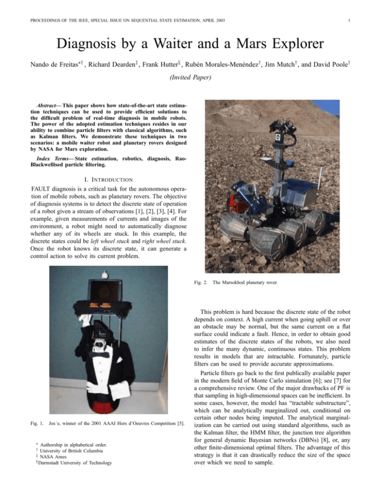
Fig. 1.
?
Jos´e, winner of the 2001 AAAI Hors d’Oeuvres Competition [5].
Authorship in alphabetical order.
University of British Columbia
‡ NASA Ames
§ Darmstadt University of Technology
†
Particle filters go back to the first publically available paper
in the modern field of Monte Carlo simulation [6]; see [7] for
a comprehensive review. One of the major drawbacks of PF is
that sampling in high-dimensional spaces can be inefficient. In
some cases, however, the model has “tractable substructure”,
which can be analytically marginalized out, conditional on
certain other nodes being imputed. The analytical marginalization can be carried out using standard algorithms, such as
the Kalman filter, the HMM filter, the junction tree algorithm
for general dynamic Bayesian networks (DBNs) [8], or, any
other finite-dimensional optimal filters. The advantage of this
strategy is that it can drastically reduce the size of the space
over which we need to sample.
PROCEEDINGS OF THE IEEE, SPECIAL ISSUE ON SEQUENTIAL STATE ESTIMATION, APRIL 2003
Marginalizing out some of the variables is an example of the
technique called Rao-Blackwellisation, because it is related to
the Rao-Blackwell formula: see [9] for a general discussion.
Rao-Blackwellised particle filters (RBPF) have been applied
in specific contexts such as mixtures of Gaussians [10],
[11], [12], fixed parameter estimation [13], HMMs [11], [12],
Dirichlet process models [14], and DBNs [8]. An excellent
theoretical treatment of the algorithms adopted in this paper
is presented in [15].
In the paper, we also propose a version of RaoBlackwellised particle filtering that does one-step look-ahead
to select good sampling regions. We show that the overhead
of the extra processing per particle of this more sophisticated
method is more than compensated by the decrease in error and
variance.
We begin the paper by presenting the mathematical models
and various particle filtering algorithms. Next, we demonstrate
our algorithms for state estimation on three robots: a Real
World Interfaces B-14 mobile robot with a B-12 base (see
Figure 1), a K-9 planetary rover (Figure 15) and a Marsokhod
planetary rover (Figure 2).
II. M ATHEMATICAL M ODEL
We represent the complex nonlinear process (robot system)
with a dynamic mixture of linear processes. In addition to
the continuous state variables corresponding to each linear
process, we have a discrete state variable that determines the
linear regime of operation. In the fault diagnosis setting, each
regime corresponds to a particular fault. Different regimes
could, however, be used to represent levels of the fault or
different internal states of the robot for the purposes of
controlling it automatically. We acquire data for each regime
separately. This data enables us to do off-line identification
with the EM algorithm [16], [17]. The models estimated with
EM are validated on test set data to ensure that we have
captured the behaviour of the process adequately. In addition,
we ensure that the data generated by the models is statistically
similar to the real data; see [18] for more details on how this
is done.
Once the stationary parameters have been identified, realtime Rao-Blackwellised particle filtering (RBPF) algorithms
are used to estimate the continuous and discrete states of the
system on-line. These estimates are used to determine the type
of fault and control policies.
In mathematical terms, we adopt the following state space
representation 1 :
zt
∼ P (zt |z0:t−1 , x0:t−1 , y1:t−1 , u1:t−1 )
xt
yt
= A(zt )xt−1 + B(zt )wt + F (zt )ut
= C(zt )xt + D(zt )vt + G(zt )ut ,
1 NOTATION: For a generic vector θ, we adopt the notation θ
1:t ,
(θ1 , θ2 , . . . , θt )0 to denote all the entries of this vector at time t. For
simplicity, we use θt to denote both the random variable and its realisation.
Consequently, we express continuous probability distributions using p (dθ t )
instead of Pr (θt ∈ dθt ) and discrete distributions using p (θt ) instead
of Pr (θt = θt ). If these distributions admit densities with respect to an
underlying measure µ (counting or Lebesgue), we denote these densities by
p (θt ). For example, when considering the space Rn , we will use the Lebesgue
measure, µ = dθt , so that P (dθt ) = p (θt ) dθt .
2
where,
•
•
•
•
•
•
•
•
yt ∈ Rny denotes the measurements.
xt ∈ Rnx denotes the unknown continuous states.
ut ∈ U is a known control signal.
zt ∈ {1, . . . , nz } denotes the unknown discrete states
(normal operation and faulty conditions).
The noise processes are i.i.d Gaussian: wt ∼ N (0, I) and
vt ∼ N (0, I).
The parameters (A, B, C, D, F, G) are identified matrices
with D(zt )D(zt )T > 0 for any zt . Typically, these
matrices are estimated with the EM algorithm for linear
dynamic systems [16]. That is, one simply fixes z and
obtains data from the physical process. With z known,
it is straightforward to estimate these matrices from the
measured data using the EM algorithm. We have to repeat
this process for each possible value of z.
The initial states are x0 ∼ N (µ0 , Σ0 ) and z0 ∼ p(z0 ).
The transition kernel P (zt |z0:t−1 , x0:t−1 , y1:t−1 ) could
correspond to either a discrete Markov transition matrix
P (zt |zt−1 ), a continuous transition density, a DBN with
some independence structure that could be exploited,
a hierarchical parameterised model, etc. The important
thing is that we can easily derive particle filters using this
very general expression for the kernel. In our experiments
we adopted a Markov transition matrix. Our model is
therefore a jump Markov linear Gaussian (JMLG) model.
For clarity of presentation, we state explicitly that our model
implies the continuous densities:
p(xt |zt , xt−1 , ut ) = N (A(zt )xt−1 + F (zt )ut , B(zt )B(zt )T )
p(yt |xt , zt , ut ) = N (C(zt )xt + G(zt )ut , D(zt )D(zt )T ).
For ease of presentation, we also drop the control signal u
from the argument of the various probability distributions.
We should notice that for each realization of zt , we have a
single linear-Gaussian model. If we knew zt , we could solve
for xt exactly using the Kalman filter algorithm. The directed
acyclic graphical model representation of our model is shown
in Figure 3.
Fig. 3. Probabilistic graphical model. Note that by conditioning on z, we
have a simple linear-Gaussian graphical model.
PROCEEDINGS OF THE IEEE, SPECIAL ISSUE ON SEQUENTIAL STATE ESTIMATION, APRIL 2003
The aim of the analysis is to compute the marginal posterior distribution of the discrete states p (z0:t |y1:t ). This
distribution can be derived from the posterior distribution
p (dx0:t , z0:t |y1:t ) by standard marginalisation. The posterior
density satisfies the following recursion
p (x0:t , z0:t |y1:t ) = p (x0:t−1 , z0:t−1 |y1:t−1 )
p (yt |xt , zt ) p (xt , zt |x0:t−1 , z0:t−1 , y1:t−1 )
(1)
×
p (yt |y1:t−1 )
This recursion involves intractable integrals in the denominator. One, therefore, has to resort to some form of numerical
approximation scheme.
III. PARTICLE F ILTERING
The idea of Monte Carlo simulation is to draw an i.i.d.
set of samples {x(i) }N
i=1 from a target distribution p(dx|y)
defined on a high-dimensional space X (for simplicity, we are
ignoring z for the time being). These N samples can be used
to approximate the target density with the following empirical
point-mass function
N
1 X
PbN ( dx0:t | y1:t ) =
δ (i) (dx0:t )
N i=1 x0:t
where δx(i) (dx) denotes the delta-Dirac mass located at x(i) .
That is, we are simply approximating a complex distribution
with a histogram of the samples as shown in Figure 4.
Target distribution
Approximation
Samples
Fig. 4. Approximating the target distribution using a histogram of the Monte
Carlo samples in a simple one-dimensional example.
3
Let us introduce an arbitrary so-called importance sampling
distribution (also often referred to as the proposal distribution
or the importance function) q ( x0:t | y1:t ). Assuming that we
want to evaluate I (f ) then, provided that the support of
q ( x0:t | y1:t ) includes the support of p ( x0:t | y1:t ), we get the
following identity
R
f (x0:t ) w
e (x0:t ) q ( x0:t | y1:t ) dx0:t
R
I (f ) =
w
e (x0:t ) q ( x0:t | y1:t ) dx0:t
where w (x0:t ) is known as the importance weight
w
e (x0:t ) =
p ( x0:t | y1:t )
q ( x0:t | y1:t )
Consequently, if oone can simulate N i.i.d. particles
n
(i)
x0:t , i = 1, ..., N according to q ( x0:t | y1:t ), a possible
Monte Carlo estimate of I (f ) is
PN
(i)
(i)
1
N
f
x
w
e
x
X
0:t
0:t
i=1
N
(i)
(i)
IbN (f ) =
=
f
x
0:t wt
PN
(i)
1
w
e
x
i=1
0:t
j=1
N
(i)
where the normalized importance weights wt
(i)
w
e x0:t
(i)
wt = P
(j)
N
e x0:t
j=1 w
are given by
(2)
For N finite, IbN () is biased (ratio of two estimates) but
asymptotically, under weak assumptions, the strong law of
a.s.
large numbers applies, that is IbN (f ) −→ I (f ). Under
N →+∞
additional assumptions a central limit theorem, with a convergence rate independent of the dimension of the integrand, can
be obtained [19]. It is clear that this integration method can
also be interpreted as a sampling method where the posterior
distribution p ( x0:t | y1:t ) is approximated by
PbN ( dx0:t | y1:t ) =
N
X
i=1
(i)
wt δx(i) (dx0:t )
(3)
0:t
A recursive (sequential in time) procedure may be obtained
Consequently, one can approximate any integrals (expectaby adopting the following proposal distribution:
tions such as the mean and variance of x) I (f ) with tractable
sums IN (f ) that converge as follows
q ( x0:t | y1:t ) = q ( x0:t−1 | y1:t−1 ) q ( xt | x0:t−1 , y1:t )
Z
N
X
1
a.s.
(i)
IN (f ) =
f (x0:t ) −−−−→ I (f ) = f (x0:t )p(dx0:t |y1:t ). and only proposing candidates xt at time t. That is the past is
N →∞
N i=1
not changed. From equation (1) (ignoring z), it is easy to see
that this importance function allows us to obtain the following
That is, the estimate IN (f ) is unbiased and by the strong
recursive estimate of the importance weights at time t:
law of large numbers, it will almost surely
converge to
(a.s.)
(i)
(i)
(i) (i)
I (f ). From the set of random samples x ; i = 1, ..., N ,
p yt | xt p xt x0:t−1 , y1:t−1
(i)
one can easily estimate any quantity I (f ) and the rate of
wt ∝
(4)
(i) (i)
q( xt x0:t−1 , y1:t )
convergence of this estimate is independent of the dimension
of the integrand. In contrast, any deterministic numerical
In our JMLG model setting, we use a weighted set of
integration method has a rate of convergence decreasing as the
(i) (i)
(i) N
dimension of the integrand increases. Unfortunately, it is usu- samples (particles) {(x0:t , z0:t ), wt }i=1 to approximate the
ally impossible to sample efficiently from the posterior density posterior with the following point-mass distribution
p ( x0:t | y1:t ) at any time t, p ( x0:t | y1:t ) being multivariate, non
N
X
(i)
standard and only known up to a proportionality constant. So
PbN (dx0:t , z0:t |y1:t ) =
wt δx(i) ,z(i) (dx0:t , z0:t ),
0:t 0:t
we turn to importance sampling.
i=1
PROCEEDINGS OF THE IEEE, SPECIAL ISSUE ON SEQUENTIAL STATE ESTIMATION, APRIL 2003
4
where δx(i) ,z(i) (dx0:t , z0:t ) denotes the Dirac-delta function.
0:t
0:t
(i)
(i)
Given N particles {x0:t−1 , z0:t−1 }N
i=1 at time t − 1, approx(i)
(i)
imately distributed according to p(dx0:t−1 , z0:t−1 |y1:t−1 ), PF
(i) (i)
enables us to compute N particles {x0:t , z0:t }N
i=1 approxi(i) (i)
mately distributed according to P (dx0:t , z0:t |y1:t ), at time t.
Since we cannot sample from the posterior directly, the PF update is accomplished by introducing an appropriate importance
proposal distribution q(dx0:t , z0:t ) from which we can obtain
samples. The basic algorithm, Figure 5 (see Figure 6 for a
graphical representation), consists of two steps: sequential importance sampling and a selection that allows us to choose the
fittest particles at each time step (see the introductory chapter
in [7] for a more detailed explanation of particle filters). This
algorithm uses the transition priors as proposal distributions;
q(x0:t , z0:t |y1:t ) = p(xt |xt−1 , zt )p(zt |z0:t−1 , x0:t−1 , y1:t−1 ).
For the selection step, we used a state-of-the-art minimum
variance resampling algorithm [20].
Sequential importance sampling step
•
For i = 1, ..., N , sample from the transition priors
(i)
∼
(i)
∼
”
zbt
(i)
(i)
(i)
P (dxt |xt−1 , zt )
”
“
“
(i)
(i) (i)
(i)
(i) (i)
bt , zbt , x0:t−1 , z0:t−1 .
and set x
b0:t , zb0:t , x
For i = 1, ..., N , evaluate and normalize the importance
weights
“
”
(i)
(i) (i)
wt ∝ p yt |b
xt , zbt
x
bt
•
(i)
P (zt |z0:t−1 , x0:t−1 , y1:t−1 )
Selection step
•
Sampled particles
Weighted particles
Resampled particles at time t
Fig. 6. Graphical representation of the PF algorithm for a continuous onedimensional problem. Starting with the resampled particles at t − 1, a new
set of particles is proposed at time t. We compute the importance weight of
each particle. Finally, we select the fittest particles according to their weights.
Note the filter has failed to track the two modes appearing on the right of the
filtering posterior distribution at time t.
If equation (1) does not admit a closed-form expression,
then equation (5) does not admit one either and samplingbased methods are still required. (Also note that the term
p (yt |y1:t−1 , z0:t ) in equation (5) does not simplify to p (yt |zt )
because there is a dependency on past values through x0:t .)
This is immediately apparent if we look at the graphical model
representation in Figure 3.
Now assuming that we can use a weighted set of samples
(i)
(i)
{z0:t , wt }N
i=1 to represent the marginal posterior distribution
PbN (z0:t |y1:t ) =
N
X
(i)
wt δz(i) (z0:t ),
0:t
i=1
the marginal density of x0:t is a Gaussian mixture
Multiply/Discard particles
n
(i)
(i)
x
b0:t , zb0:t
(i)
high/low importance weights wt
o
n
(i) (i) N
.
x0:t , z0:t
oN
with respect to
i=1
to obtain N particles
i=1
Fig. 5.
Resampled particles at time t−1
pbN (x0:t |y1:t )
=
Z
p(x0:t |z0:t , y1:t )dP (z0:t |y1:t )
=
Z
p(x0:t |z0:t , y1:t )
=
PF algorithm at time t.
N
X
(i)
wt δz(i) (z0:t )
0:t
i=1
N
X
(i)
(i)
wt p(x0:t |y1:t , z0:t )
(6)
i=1
IV. R AO -B LACKWELLISED PARTICLE F ILTERING
By considering the following factorization [9]:
p ( x0:t , z0:t | y1:t ) = p ( x0:t | y1:t , z0:t ) p ( z0:t | y1:t ) ,
it is possible to design algorithms with less variance. The
density p ( x0:t | y1:t , z0:t ) is Gaussian (given zt , the JMLG
model reduces to a simple linear Gaussian model) and can
be computed analytically if we know the marginal posterior
density p ( z0:t | y1:t ). This density satisfies the alternative recursion
p (z0:t |y1:t ) = p (z0:t−1 |y1:t−1 )
p (yt |y1:t−1 , z0:t ) p (zt |z0:t−1 , y1:t−1 )
×
p (yt |y1:t−1 )
that can be computed efficiently with a stochastic bank of
Kalman filters. That is, we use PF to estimate the distribution
of zt and exact computations (Kalman filters — one for
each particle) to estimate the mean and variance of xt . In
(i)
(i)
particular, we sample zt and then propagate the mean µt
(i)
and covariance Σt of xt with a Kalman filter:
(i)
(i)
(i)
(i)
(i)
(i)
(i)
(i)
(i)
(i)
(i)
(i)
(i)
Σt|t−1 = A(zt )Σt−1 A(zt )T + B(zt )B(zt )T
(i)
St
(i)
(i)
(i)
= C(zt )Σt|t−1 C(zt )T + D(zt )D(zt )T
(i)
(i)
yt|t−1 = C(zt )µt|t−1 + G(zt )ut
(i)
(i)
(i)
−1(i)
(i)
(i)
(i)
−1(i)
(i)
= µt|t−1 + Σt|t−1 C(zt )T St
(i)
= Σt|t−1 − Σt|t−1 C(zt )T St
µt
(5)
(i)
µt|t−1 = A(zt )µt−1 + F (zt )ut
Σt
(i)
(yt − yt|t−1 )
(i)
(i)
C(zt )Σt|t−1 ,
PROCEEDINGS OF THE IEEE, SPECIAL ISSUE ON SEQUENTIAL STATE ESTIMATION, APRIL 2003
V. L OOK -A HEAD R AO -B LACKWELLISED PARTICLE
F ILTERING
where,
•
•
•
•
•
•
µt|t−1 , E ( xt | y1:t−1 )
µt , E ( xt | y1:t )
y t|t−1 , E ( yt | y1:t−1 )
Σt|t−1 , cov ( xt | y1:t−1 )
Σt , cov ( xt | y1:t )
St , cov ( yt | y1:t−1 ).
In order to deal with unexpected observations, it is possible
to improve the RBPF by looking one step ahead. One can
expand the expression for the importance weights as follows:
wt
Hence, using the prior proposal for zt and applying equation
(5), we find that the importance weights for zt are given by
the predictive density
p ( yt | y1:t−1 , z1:t ) = N yt ; y t|t−1 , St .
(7)
This RBPF algorithm was applied to fault diagnosis in [21].
The algorithm is shown in Figure 7.
Sequential importance sampling step
•
•
(i)
(i)
(i)
b (i)
For i = 1, ..., N , set µ
b t|t−1 , µ t|t−1 , Σ
t|t−1 , Σ t|t−1 ,
sample
(i)
zbt
∼
(i)
(i)
Pr(zt |x0:t−1 , z0:t−1 , y1:t−1 )
For i = 1, ..., N , evaluate and normalize the importance weights
“
”
(i)
(i)
wt ∝ p yt |y1:t−1 , zbt
Selection step
•
=
=
∝
p(z0:t |y1:t )
q(z0:t |y1:t )
p(z0:t−1 |y1:t ) p(zt |z0:t−1 , y1:t )
p(z0:t−1 |y1:t−1 ) q(zt |z0:t−1 , y1:t )
p (yt |y1:t−1 , z0:t ) p (zt |z0:t−1 , y1:t−1 )
.
q (zt |z0:t−1 , y1:t )
(8)
(9)
(10)
The choice of proposal distribution, q(z0:t |y1:t )
=
q(zt |z0:t−1 , y1:t )p(z0:t−1 |y1:t−1 ), states that we are not
sampling past trajectories. Sampling past trajectories requires
solving an intractable integral [22].
We could use the transition prior as proposal distribution:
q(zt |z0:t−1 , y1:t ) = p (zt |z0:t−1 , y1:t−1 ). Then, according to
equation (10), the importance weights simplify to the predictive density of equation (7).
However, according to equation (9), the optimal proposal
distribution corresponds to the choice q(zt |z0:t−1 , y1:t ) =
p(zt |z0:t−1 , y1:t ). This distribution satisfies Bayes rule:
p (yt |y1:t−1 , z0:t ) p (zt |z0:t−1 , y1:t−1 )
p (yt |y1:t−1 , z0:t−1 )
(11)
and, hence, the importance weights simplify to
p (zt |z0:t−1 , y1:t ) =
wt ∝ p (yt |y1:t−1 , z0:t−1 )
nz
X
p (yt |y1:t−1 , z0:t−1 , zt ) p (zt |z0:t−1 , y1:t−1 ) (12)
∝
zt =1
n
oN
(i)
b (i) , zbt(i)
with
Multiply/Discard particles µ
bt|t−1 , Σ
t|t−1
i=1
(i)
respect to high/low
importanceoweights wt
n
N
(i)
(i)
(i)
.
N particles µt|t−1 , Σt|t−1 , zt
to obtain
i=1
Updating step
•
5
For i
=
1, ..., N , use one step of the
Kalman recursion
to compute the o sufficient
n
(i)
(i)
(i)
(i)
statistics
µ t+1|t , Σ t+1|t , yt+1|t , St+1 ,
given
n
o
(i)
(i)
(i)
zt , µ t|t−1 , Σ t|t−1 .
(i)
Fig. 7. RBPF algorithm at time t. For each particle zt we propagate the
mean and variance of xt . This enables us to approximate the posterior of
x with a mixture of Gaussians. Note that in the simple PF, the posterior is
approximated with a more coarse model: a mixture of Dirac-delta functions.
The RBPF requires that we propagate a Kalman filter for
each particle. It appears at first sight to be computational
expensive. The experiments will show, however, that this extra
computation per particle can result in vast improvements in
accuracy and robustness.
When the number of discrete states is small, say 10 or
1000, we can compute the distributions in equations (11) and
(12) analytically. That is, if the number of discrete states
is reasonably small, we can compute the sums by simple
enumeration. In addition to Rao-Blackwellization, this leads
to substantial improvements over standard particle filters. Yet,
a further improvement can still be attained.
Even when using the optimal importance distribution, there is a discrepancy arising from the ratio
p(z0:t−1 |y1:t )/p(z0:t−1 |y1:t−1 ) in equation (9). This discrepancy is what causes the well known problem of sample
impoverishment in all particle filters [7], [23]. To circumvent
it to a significant extent, one can note that the importance
weights do not depend on zt (we are marginalising over this
variable). It is therefore possible to select particles before
the sampling step. That is, one chooses the fittest particles
at time t − 1 using the information at time t. This leads to
an efficient algorithm (look-ahead RBPF), [15], [2] , whose
pseudocode is shown in Figure 8. Note that for standard
PF, Figure 5, the importance weights depend on the sample
(i)
zt , thus not permitting selection before sampling. Selecting
particles before sampling results in a richer sample set at
the end of each time step. See Figure 9 for a graphical
representation.
PROCEEDINGS OF THE IEEE, SPECIAL ISSUE ON SEQUENTIAL STATE ESTIMATION, APRIL 2003
6
Sampled particles at time t−1
Kalman prediction step
•
•
Weighted particles
Resampled particles
For i=1, . . . , N, and for zt = 1, . . . , nz compute
(i)
b (i) (zt ), yb(i) (zt ), S
b(i) (zt )
µ
bt|t−1 (zt ), Σ
t
t|t−1
t|t−1
For i=1 , . . . , N , evaluate and normalize the importance
weights
(i)
=
wt
=
(i)
p(yt |y1:t−1 , z0:t−1 )
nz
X
zt =1
(i)
b(i) (zt ))p(zt |z (i) , y1:t−1 )
N (b
yt|t−1 (zt ), S
t
0:t−1
Fig. 9. Graphical representation of look-ahead RBPF. First we compute the
importance weights. After resampling according to these weights, we propose
new particles at time t. With this algorithm, we are more likely to be able to
track all the modes of the changing filtering distribution.
Selection step
•
Multiply/Discard particles
n
(i) b (i)
(i)
µ
bt−1 , Σ
b0:t−1
t−1 , z
respect to high/low importance weights
n
oN
(i)
(i)
(i)
.
particles µt−1 , Σt−1 , z0:t−1
(i)
wt
oN
i=1
with
to obtain N
i=1
Sequential importance sampling step
•
•
Kalman prediction. For i=1, . . . , N, and for zt = 1, . . . , nz
using the resampled information, re-compute
(i)
b (i) (zt ), yb(i) (zt ), S
b(i) (zt )
µ
bt|t−1 (zt ), Σ
t
t|t−1
t|t−1
For zt = 1, . . . , nz compute
(i)
(i)
(i)
(i)
p(zt |z0:t−1 , y1:t ) ∝ N (b
yt|t−1 (zt ), Sbt (zt ))p(zt |z0:t−1 , y1:t−1 )
•
Sampling step
(i)
zt
(i)
∼ p(zt |z0:t−1 , y1:t )
Updating step
•
For i=1 , . . . , N, use one step of the Kalman
recursion
compute
the
sufficient o statistics
o to
n
n
(i) b
(i)
(i)
(i)
given µ
bt|t−1 (zt ), Σ
µt , Σ t
t|t−1 (zt ) .
Fig. 8.
Look-ahead RBPF algorithm at time t. The algorithm uses an
optimal proposal distribution. It also selects particles from time t − 1 using
the information at time t.
VI. E XPERIMENTS
WITH
Sampled particles at time t
The B-12’s motors are stepping motors, controlled by a
varying pulse width. Actual translation and rotational speed
are measured by optical shaft encoders - one for translation
and one for rotation. Individual wheels do not have separate
encoders, so are assumed to all be translating or rotating at
the same speed. There are commands to set the desired speed
and acceleration. A feedback control loop monitors the actual
values and adjusts the motor pulse width to achieve the desired
values. Simpler open-loop commands are also available - these
bypass the control loop and send a fixed pulse width directly
to the motors.
The B-12 provides status reports including measured translational and rotational speeds, current and pulse width to either
motor, battery voltage, etc. Jos´e also has a stereo camera and
bump, infrared, and sonar sensors.
A. Experimental Setup
Using the currents as control signals ut , we measured the
speeds of the wheels yt . We used a one dimensional continuous
state xt . This state need not have a physical interpretation (this
is indeed not needed in our fault diagnosis setting). It should
rather be interpreted as a projection of yt to a noiseless space.
We performed tests using two sets of four discrete states zt ,
chosen as follows:
B-14 R ESEARCH ROBOT
Jos´e is a general purpose research robot, specifically a Real
State Description
World Interfaces B-14 mobile robot with a B-12 base, who
1
Smooth floor, no extra load
recently won the AAAI Hors d’Oeuvres Competition [5] (see
2
Smooth floor, dragging a light load
Figure 1).
3
Smooth floor, dragging a medium load
The base unit contains two separate motors, one for transla4
Smooth floor, dragging a heavy load
tion and one for rotation. Power is provided by a rechargeable
5
Tiled floor, no extra load
battery. The translational motor drives all three wheels, giving
6
Tiled floor, dragging a light load
excellent traction. The rotational motor turns all three wheels
7
Tiled floor, dragging a medium load
in unison, so they are always pointing the same way. Thus
8
Tiled floor, dragging a heavy load
there is no concept of ”front” or ”back” wheels - a given
wheel can end up in the front (relative to the direction of
The ’dragging’ states were chosen so that we could repeattravel), at the back, or anywhere in between. Jos´e can move
along curved paths by simultaneously translating and rotating. ably simulate a fault situation in which Jos´e has bumped into
PROCEEDINGS OF THE IEEE, SPECIAL ISSUE ON SEQUENTIAL STATE ESTIMATION, APRIL 2003
100
90
80
% Error Detection
or snagged something. The smooth floor represents a lownoise environment, while the tiled floor represents a noisy
environment.
We engineered the initial and transition matrices for the
discrete states z0 ∼ p(z0 ) and p(zt |zt−1 ), collected data in
each discrete state and learned the matrices A, C, F, G using
a conventional optimization process and a standard procedure
in control engineering [24]. The noise matrices B and D were
learned via the expectation maximisation (EM) algorithm for
linear dynamic models [16]. Figure 10 shows the measured
data and data generated by the JMLG model under several
step responses.
7
PF
70
60
50
RBPF
40
30
la−RBPF
20
10
5
High
0
4
0
1
10
Zt
Low
Low
2
0
0
Medium
Normal
10
100
200
300
time (=) 1/10 sec
400
Fig. 11. Smooth floor. Diagnosis error vs number of particles. Estimation
based on 25 runs.
500
100
90
0.7
Real data
Real time
80
0.6
0.5
0.4
JMLG model
0.3
0
100
200
300
time (=) 1/10 sec
400
500
% Error Detection
Speed (=) m/s
3
10
Number of particles
3
1
2
10
70
PF
60
50
40
RBPF
30
Fig. 10. To test how well our models capture the behaviour of the data, we
used them to generate data under a switching load zt . As shown in the plot
below, the generated data yt captures the trends in the real data.
20
10
la−RBPF
0 −3
10
−2
−1
0
10
10
10
Computing time per timestep (=) sec
1
10
B. Testing and Results
Over 30 test runs were conducted, in which the robot
was placed in different states at random times. Measurements
were recorded every 0.1 sec. The three particle filtering
algorithms were tested. For each dataset and algorithm, we
plotted diagnosis error rate versus number of particles and
CPU time. The diagnosis error rate is the percentage of time
steps in which the diagnosed state differed from the actual
state. This obviously decreases with the number of particles in
all algorithms. Note that there is a baseline error rate resulting
from human inaccuracy in timing the state changes.
1) Low-Noise Environment: Test runs involving state
changes while the robot was travelling on the smooth floor
produced the results shown in figures 12 and 11. In this
environment, la-RBPF is clearly superior. One would expect
it to perform better than the other algorithms for the same
number of particles; la-RBPF is doing a lot more work per
particle. But even when the extra time per particle is factored
in, la-RBPF is still more efficient. Overall it produces a lower
Fig. 12. Smooth floor. Diagnosis error vs computing time. Estimation based
on 25 runs.
error rate (and lower variance) than PF and RBPF using the
same CPU time.
2) High-Noise Environment: Similar state changes while
operating on a tiled floor yielded different results (see Figure 13). Here, la-RBPF’s extra work resulted in no benefit.
When we applied a simple moving-average filter to the data,
la-RBPF’s advantage was restored – Figure 14.
VII. E XPERIMENTS
WITH
M ARS ROVERS
A. K-9 rover
We performed experiments on a simple model of the suspension system of the K-9 rover at NASA Ames Research Center.
K-9, shown in Figure 15, is a six wheeled rover with a rockerbogey suspension, and we model the suspension’s response to
PROCEEDINGS OF THE IEEE, SPECIAL ISSUE ON SEQUENTIAL STATE ESTIMATION, APRIL 2003
8
100
90
% Error Detection
80
Real time
RBPF
70
60
50
PF
la−RBPF
40
30
20
10
0
−3
−2
10
10
−1
10
0
10
1
10
Computing time per timestep (=) sec
Fig. 13. Tiled floor. Diagnosis error vs computing time. Estimation based
on 25 runs.
100
90
Real time
% Error Detection
80
70
60
50
40
PF
30
RBPF
20
10
0
la−RBPF
−3
10
Fig. 15.
−2
10
−1
10
0
10
The planetary rover K-9.
1
10
Computing time per timestep (=) sec
Fig. 14. Tiled floor. Diagnosis error vs computing time, where the measurement signals have been filtered (smoothed). Estimation based on 25 runs.
driving over rocks and other obstacles to anticipate situations
where the rover’s scientific instruments could collide with an
obstacle, or where the rover could become “high-centered”
on a rock. The model has six discrete modes that refer to flat
driving, rock under front wheel, rock under middle wheel, rock
under rear wheel, rock between front and middle wheel and
rock between middle and rear wheel, respectively. There are
four continuous parameters in the model, which represent the
rocker and bogey angles and their derivatives. The angles are
the two observable variables of the system.
The trajectories of rocker and bogey angles α and β can be
modelled as trigonometric functions when one wheel is going
over the rock and constant otherwise. By also modelling their
derivatives α̇ and β̇ as continuous parameters of the system,
we obtain linear probabilistic transition functions of the form
αt = αt−1 + k α̇t−1 + N (0, σα2 )
and
α̇t = αt−1
˙ + k αt−1
¨ + N (0, σα̇2 )
and likewise for β. With α̈t = −αt in the trigonometric
case and α̈t = 0 in the constant case all transition functions
are linear functions of the system’s continuous parameters.
The discrete transition function and the noise terms were
engineered by hand.
We carried out two sets of tests. In the first set, the model
was used to generate data for which ground truth was available
as to the true values of the mode and continuous variables, and
the algorithms were applied to this artificial data. In the second
setting, we applied the model to detect rocks in real data. This
data was generated at NASA Ames by driving the K-9 rover
over three different rocks in an outdoor “sandbox” consisting
of gravel, sand, rocks and small hills.
We first report the results on artificial data with ground truth.
Here, the look-ahead variant of RBPF proved to be highly
efficient. In this set of tests, the diagnosis of every filter is
taken to be the maximum a posteriori (MAP) estimate of the
discrete modes.
PROCEEDINGS OF THE IEEE, SPECIAL ISSUE ON SEQUENTIAL STATE ESTIMATION, APRIL 2003
9
0
90
10
80
−1
10
70
PF
−2
PF
Mean squared error
% Error detection
60
10
50
40
30
RBPF
−4
10
RBPF
20
10
−3
10
−5
10
la−RBPF
−6
10
0
la−RBPF
−7
−10
0
10
1
2
10
3
10
10
Number of particles
Fig. 16.
runs.
Performance of PF, RBPF and la-RBPF. Estimation based on 50
10
−2
10
−1
0
10
10
Computing time per timestep (=) sec
1
10
Fig. 18. Mean squared errors of the PF, RBPF and la-RBPF algorithms,
averaged over 50 runs. Note the logarithmic scale for both the X- and Yaxes.
90
80
real time
70
% Error detection
60
50
40
30
RBPF
20
10
PF
la−RBPF
0
−10
−2
10
Fig. 17.
runs.
−1
0
10
10
Computing time per timestep (=) sec
1
10
Performance of PF, RBPF, and la-RBPF. Estimation based on 50
Figure 16 shows the percentage of incorrect diagnoses for
PF, RBPF, and la-RBPF for a varying number of particles.
Clearly, la-RBPF and RBPF yield better results than PF with
the same number of particles. When we take into account
the additional computation time la-RBPF and RBPF need per
particle, the performance of PF and RBPF is comparable but
the two are still clearly dominated by la-RBPF (see Figure 17).
In some cases we are not only interested in diagnosing the
discrete modes, but also the continuous parameters of a hybrid
system. As an example we might want to know the steepness
of a hill, or the size of a rock we are driving over. In other
applications, these continuous parameters might be crucial,
particularly when diagnosing sensor defects and calibration
problems.
Figure 18 shows the mean squared error (MSE) of the PF,
RBPF and la-RBPF algorithms on the same artificial data
as above where ground truth is available. The Y-scale is
logarithmic to fit the extreme differences between PF and the
other algorithms. With a mean squares estimation error of the
continuous parameters which is between 103 and 105 times
higher than that of la-RBPF, it is clearly outperformed. The
difference between RBPF and la-RBPF is very small with
the look-ahead variant performing slightly better for small
numbers of particles.
We also applied the algorithms to real data from the K9 rover. In Figure 19, we show the two observed variables,
rocker and bogey angle as well as the discrete mode estimates
PF and la-RBPF yield with the number of particles they can
roughly process in real time. PF uses 32 particles while laRBPF is allowed to use 4 particles. To avoid a cluttered picture
we omit RBPF (with eight particles) which yields better results
than PF but still performs worse than la-RBPF. To iterate, state
1 represents flat driving, state 2 driving over a rock with the
front wheel, state 3 with the middle wheel and state 4 with the
rear wheel. State 5 represents the rock being between the front
and the middle wheel and state 6 between the middle and the
rear wheel. There is no ground truth for this data, although it is
fairly clear from the data when the rover drives over the three
rocks. The PF almost misses the third rock and gets confused
by little changes in the data during flat driving. The la-RBPF
algorithm detects all the rocks and only the rocks, but on the
second rock, the traversal of the rear wheel is missed. We
believe this is due to weaknesses in the model rather than in
the tracking algorithm.
B. Marsokhod rover
At NASA Ames Research Center, we also applied RaoBlackwellised Particle Filtering for model-based fault detection on the Marsokhod rover, a medium-sized planetary
rover with six wheels (see Figure 2). The wheel model was
initially only designed to demonstrate feasibility of model
based diagnosis [25]. It is completely hand-crafted and the
effort of tuning parameters was not undertaken. Despite this
PROCEEDINGS OF THE IEEE, SPECIAL ISSUE ON SEQUENTIAL STATE ESTIMATION, APRIL 2003
10
60
6
PF
4
Number of measurements needed
Observations and filter estimates
PF
50
5
la−RBPF
3
2
1
40
30
20
RBPF
10
Bogey angle
0
0
la−RBPF
Rocker angle
−1
0
Fig. 19.
50
100
150
Time steps
200
250
−10
0
10
300
Discrete mode estimates on real data.
1
2
10
3
4
10
10
Number of particles
5
10
10
Fig. 20. Number of measurements needed to diagnose a fault. Algorithms PF,
RBPF and la-RBPF with a varying number of particles available for diagnosis.
Estimation based on 25 runs.
90
80
real time
fact, we can diagnose faults very efficiently and correctly using
this model and Rao-Blackwellised particle filtering.
Diagnosis is run independently on each of the six wheels.
There are 22 discrete states, 9 of which are normal operational
states and 13 of which represent fault states. Diagnosable faults
include a stalled motor, a broken gear, and a broken gear and
encoder. For the experiments we describe here, the right rear
wheel had a broken gear and encoder. The task of diagnosis
was to reliably identify this fault with as little measurements
as possible. The rover was set to an idle state in which the
fault is not diagnosable and then it was given the command to
start. We report the number of measurements the algorithms
needed to settle for the diagnosis of a broken gear and encoder
at the rear back wheel.
In Figure 20, we report this number of measurements on
the Y-axis as a function of the varying number of particles
the algorithms are given (the total number of measurements
after the command was issued was 46 and if the fault is never
diagnosed we report this number). Standard Particle Filters
show very inferior performance in this task. Only with 1000
particles and above they are able to diagnose the fault in
some of the experiments. The look-ahead variant of RBPF,
on the other hand, can already diagnose the fault with one
single particle. It is simply tracking the mode very well. The
picture does not change much when we take into account
the different time complexities of the algorithms: la-RPBF is
still performing considerably better than RBPF which in turn
outperforms PF significantly. For additional information on the
wheel model and more experiments we refer the reader to [25].
Number of measurements needed
70
60
PF
50
40
30
RBPF
20
10
la−RBPF
0
−10
−3
10
−2
10
−1
0
1
10
10
10
Computing time per timestep (=) sec
2
10
3
10
Fig. 21. Number of measurements needed to diagnose a fault. Algorithms
PF, RBPF and la-RBPF with varying computation time given per time step.
Estimation based on 25 runs.
VIII. C ONCLUSION
In this paper, we demonstrated the use of algorithms, that
combine particle and Kalman filters, for diagnosing mobile
robots. In particular, we showed that the look-ahead RBPF
can compute very accurate diagnosis probabilities in real-time.
There are two reasons for this. First, marginalising continuous
variables reduces the problem of high-dimensional state spaces
considerably. Second, the look ahead feature is important
in diagnosis with particle filters, where the probability of
faulty states is typically low. Looking one step-ahead improves
the probability of proposing particles in these states of low
probability.
This state estimation method can also be used to select
control strategies [26]. This is an essential step toward having
robots that can carry out self-maintenance.
PROCEEDINGS OF THE IEEE, SPECIAL ISSUE ON SEQUENTIAL STATE ESTIMATION, APRIL 2003
There are several avenues for further research. Standard
particle filters allow us to adopt nonlinear measurement models, but this comes with a great computational cost. Many
current efforts are being devoted to the design of efficient
filters to handle this situation [27], [28], [29]. We also need to
investigate hierarchical models for specifying faults. The aim
is to end up with sparse models that can be solved efficiently
using multiple Rao-Blackwellisation. Finally, it is important
to continue testing the robots, models and algorithms in more
demanding conditions.
ACKNOWLEDGMENT
We thank the Jos´e team at UBC and, in particular, Pantelis
Elinas and Don Murray for getting us started with Jos´e.
We would also like to thank Arnaud Doucet for suggestions
and Zoubin Ghahramani for his EM code for linear dynamic
models. Nando de Freitas was supported by NSERC and IRISROPAR, Frank Hutter was partially supported by a RIACS
SSRP student fellowship at NASA Ames Research Center,
Ruben Morales-Men´endez was partially supported by the
Government of Canada (ICCS) and UBC’s CS department.
R EFERENCES
[1] S. Thrun, J. Langford, and V. Verma, “Risk sensitive particle filters,”
in Advances in Neural Information Processing Systems 14, S. B.
T. G Dietterich and Z. Ghahramani, Eds. Cambridge, MA: MIT Press,
2002.
[2] R. Morales-Menendez, N. de Freitas, and D. Poole, “Real-time monitoring of complex industrial processes with particle filters,” in Advances
in Neural Information Processing Systems 16. Cambridge, MA: MIT
Press, 2003.
[3] R. Dearden and D. Clancy, “Particle filters for real-time fault detection
in planetary rovers,” in International Workshop on Diagnosis, 2001.
[4] V. Verma, J. Fernandez, and R. Simmons, “Probabilistic models for
monitoring and fault diagnosis,” in The Second IARP and IEEE/RAS
Joint workshop on technical challenges for dependable robots in human
environment, R. Chatila, Ed., Toulouse, France, October 2002.
[5] P. Elinas, J. Hoey, D. Lahey, J. D. Montgomery, D. Murray, S. Se,
and J. J. Little, “Waiting with Jos´e, a vision-based mobile robot.” in
International Conference on Robotics and Automation, 2002.
[6] N. Metropolis and S. Ulam, “The Monte Carlo method,” Journal of the
American Statistical Association, vol. 44, no. 247, pp. 335–341, 1949.
[7] A. Doucet, N. de Freitas, and N. J. Gordon, Eds., Sequential Monte
Carlo Methods in Practice. Springer-Verlag, 2001.
[8] A. Doucet, N. de Freitas, K. Murphy, and S. Russell, “Rao-Blackwellised
particle filtering for dynamic Bayesian networks,” in Uncertainty in
Artificial Intelligence, C. Boutilier and M. Godszmidt, Eds. Morgan
Kaufmann Publishers, 2000, pp. 176–183.
[9] G. Casella and C. P. Robert, “Rao-Blackwellisation of sampling
schemes,” Biometrika, vol. 83, no. 1, pp. 81–94, 1996.
[10] H. Akashi and H. Kumamoto, “Random sampling approach to state
estimation in switching environments,” Automatica, vol. 13, pp. 429–
434, 1977.
[11] A. Doucet, “On sequential simulation-based methods for Bayesian
filtering,” Department of Engineering, Cambridge University, Tech. Rep.
CUED/F-INFENG/TR 310, 1998.
[12] A. Doucet, S. Godsill, and C. Andrieu, “On sequential Monte Carlo
sampling methods for Bayesian filtering,” Statistics and Computing,
vol. 10, no. 3, pp. 197–208, 2000.
[13] A. Kong, J. S. Liu, and W. H. Wong, “Sequential imputations and
Bayesian missing data problems,” Journal of the American Statistical
Association, vol. 89, no. 425, pp. 278–288, 1994.
[14] S. N. MacEachern, M. Clyde, and J. S. Liu, “Sequential importance sampling for nonparametric Bayes models: the next generation,” Canadian
Journal of Statistics, vol. 27, pp. 251–267, 1999.
[15] A. Doucet, N. J. Gordon, and V. Krishnamurthy, “Particle filters for
state estimation of jump Markov linear systems,” Cambridge University
Engineering Department, Tech. Rep. CUED/F-INFENG/TR 359, Sept.
1999.
11
[16] S. Roweis and Z. Ghahramani, “A unifying review of linear Gaussian
models,” Neural Computation, vol. 11, no. 2, pp. 305–345, 1999.
[17] R. H. Shumway and D. S. Stoffer, “An approach to time series smoothing
and forecasting using the EM algorithm,” Journal of Time Series
Analysis, vol. 3, no. 4, pp. 253–264, 1982.
[18] N. de Freitas, M. Niranjan, A. H. Gee, and A. Doucet, “Global
optimisation of neural network models via sequential sampling,” in
Advances in Neural Information Processing Systems, M. J. Kearns, S. A.
Solla, and D. Cohn, Eds., vol. 11, MIT Press, 1999, pp. 410–416.
[19] J. Geweke, “Bayesian inference in econometric models using Monte
Carlo integration,” Econometrica, vol. 24, pp. 1317–1399, 1989.
[20] G. Kitagawa, “Monte Carlo filter and smoother for non-Gaussian nonlinear state space models,” Journal of Computational and Graphical
Statistics, vol. 5, pp. 1–25, 1996.
[21] N. de Freitas, “Rao-Blackwellised particle filtering for fault diagnosis,”
in IEEE Aerospace Conference, 2001.
[22] C. Andrieu, A. Doucet, and E. Punskaya, “Sequential Monte Carlo
methods for optimal filtering,” in Sequential Monte Carlo Methods in
Practice, A. Doucet, N. de Freitas, and N. J. Gordon, Eds. SpringerVerlag, 2001.
[23] M. K. Pitt and N. Shephard, “Filtering via simulation: Auxiliary particle
filters,” Journal of the American Statistical Association, vol. 94, no. 446,
pp. 590–599, 1999.
[24] L. Ljung, System Identification: Theory for the User. Prentice-Hall,
1987.
[25] R. Washington, “On-board real-time state and fault identification for
rovers,” in IEEE International Conference on Robotics and Automation,
2000.
[26] R. Morales-Menendez, N. de Freitas, and D. Poole, “Estimation and
control of industrial processes with particle filters,” in American Control
Conference, 2003.
[27] C. Andrieu, M. Davy, and A. Doucet, “Efficient particle filtering for
jump markov systems,” 2003, to appear in IEEE Transactions on Signal
Processing.
[28] F. Hutter and R. Dearden, “Efficient on-line fault diagnosis for nonlinear systems,” in Proceedings of the 7th International Symposium on
Artificial Intelligence, Robotics and Automation in Space, 2003.
[29] ——, “The gaussian particle filter for diagnosis of non-linear systems,”
in Under Review for the 14th International Workshop on Principles of
Diagnosis, 2003.