The multiplier effect The “multiplier” tells us the change in
advertisement
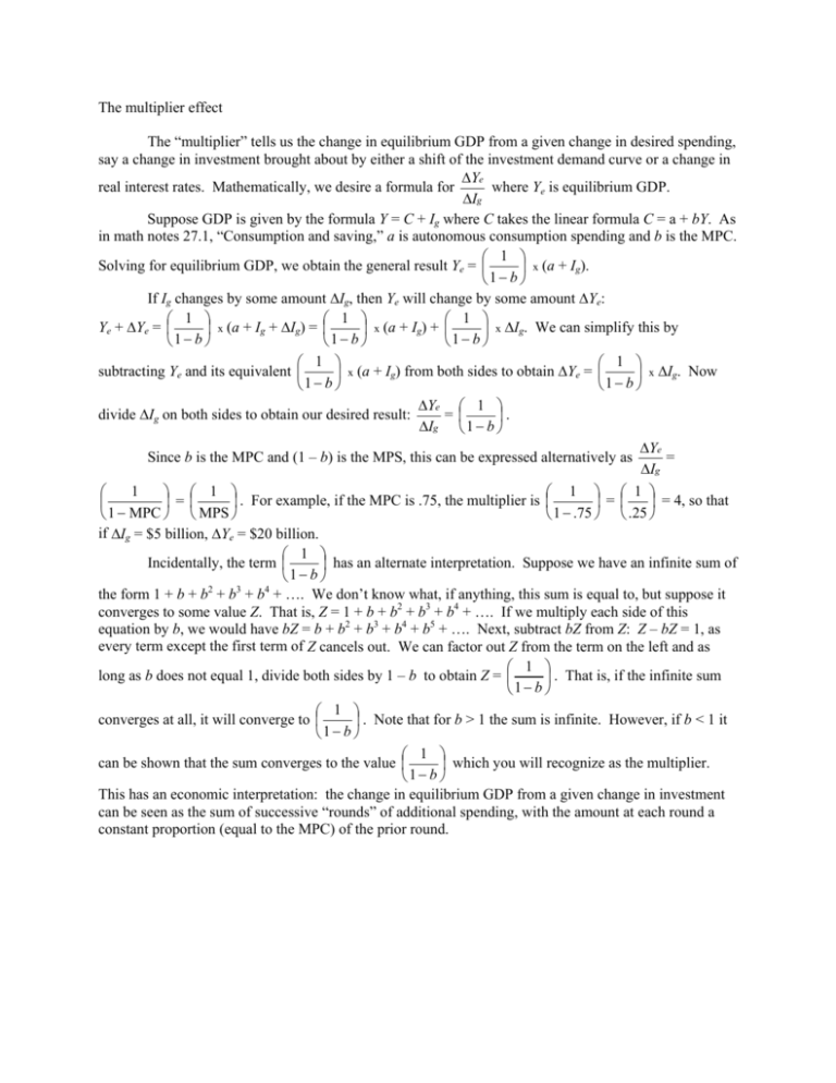
The multiplier effect The “multiplier” tells us the change in equilibrium GDP from a given change in desired spending, say a change in investment brought about by either a shift of the investment demand curve or a change in ∆Ye real interest rates. Mathematically, we desire a formula for where Ye is equilibrium GDP. ∆Ig Suppose GDP is given by the formula Y = C + Ig where C takes the linear formula C = a + bY. As in math notes 27.1, “Consumption and saving,” a is autonomous consumption spending and b is the MPC. 1 Solving for equilibrium GDP, we obtain the general result Ye = x (a + Ig). 1− b If Ig changes by some amount ∆Ig, then Ye will change by some amount ∆Ye: 1 1 1 Ye + ∆ Y e = x (a + Ig + ∆Ig) = x (a + Ig) + x ∆Ig. We can simplify this by 1 − b 1 − b 1− b 1 1 subtracting Ye and its equivalent x (a + Ig) from both sides to obtain ∆Ye = x ∆Ig. Now 1 b − 1− b ∆Ye 1 divide ∆Ig on both sides to obtain our desired result: = . ∆Ig 1 − b ∆Ye = Since b is the MPC and (1 – b) is the MPS, this can be expressed alternatively as ∆Ig 1 1 1 1 = . For example, if the MPC is .75, the multiplier is = = 4, so that 1 − MPC MPS 1 − .75 .25 if ∆Ig = $5 billion, ∆Ye = $20 billion. 1 Incidentally, the term has an alternate interpretation. Suppose we have an infinite sum of 1− b the form 1 + b + b2 + b3 + b4 + …. We don’t know what, if anything, this sum is equal to, but suppose it converges to some value Z. That is, Z = 1 + b + b2 + b3 + b4 + …. If we multiply each side of this equation by b, we would have bZ = b + b2 + b3 + b4 + b5 + …. Next, subtract bZ from Z: Z – bZ = 1, as every term except the first term of Z cancels out. We can factor out Z from the term on the left and as 1 long as b does not equal 1, divide both sides by 1 – b to obtain Z = . That is, if the infinite sum 1 − b 1 converges at all, it will converge to . Note that for b > 1 the sum is infinite. However, if b < 1 it 1− b 1 can be shown that the sum converges to the value which you will recognize as the multiplier. 1 − b This has an economic interpretation: the change in equilibrium GDP from a given change in investment can be seen as the sum of successive “rounds” of additional spending, with the amount at each round a constant proportion (equal to the MPC) of the prior round.
