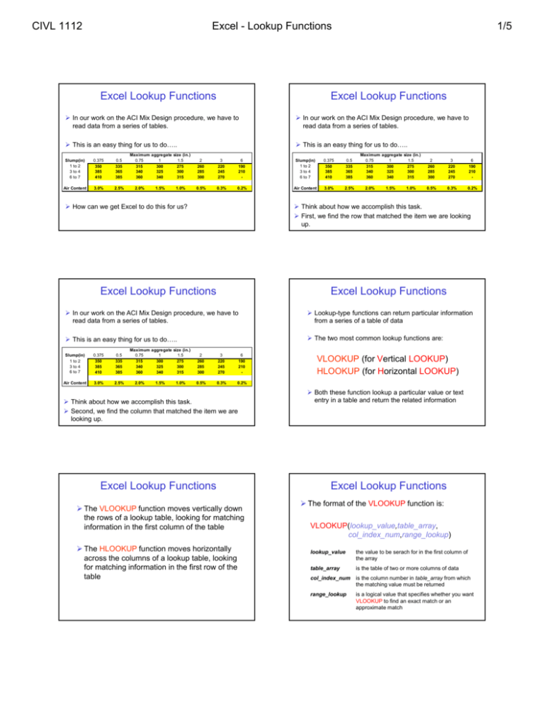
CIVL 1112
Excel - Lookup Functions
Excel Lookup Functions
1/5
Excel Lookup Functions
 In our work on the ACI Mix Design procedure, we have to
read data from a series of tables.
 In our work on the ACI Mix Design procedure, we have to
read data from a series of tables.
 This is an easy thing for us to do…..
 This is an easy thing for us to do…..
Slump(in)
1 to 2
3 to 4
6 to 7
0.375
350
385
410
0.5
335
365
385
Air Content
3.0%
2.5%
Maximum aggregate size (in.)
0.75
1
1.5
315
300
275
340
325
300
360
340
315
2.0%
1.5%
1.0%
2
260
285
300
3
220
245
270
6
190
210
-
Slump(in)
1 to 2
3 to 4
6 to 7
0.375
350
385
410
0.5
335
365
385
0.5%
0.3%
0.2%
Air Content
3.0%
2.5%
Maximum aggregate size (in.)
0.75
1
1.5
315
300
275
340
325
300
360
340
315
2.0%
1.5%
1.0%
2
260
285
300
3
220
245
270
6
190
210
-
0.5%
0.3%
0.2%
 Think about how we accomplish this task.
 First, we find the row that matched the item we are looking
up.
 How can we get Excel to do this for us?
Excel Lookup Functions
Excel Lookup Functions
 In our work on the ACI Mix Design procedure, we have to
read data from a series of tables.
 Lookup-type functions can return particular information
from a series of a table of data
 This is an easy thing for us to do…..
 The two most common lookup functions are:
Slump(in)
1 to 2
3 to 4
6 to 7
0.375
350
385
410
0.5
335
365
385
Air Content
3.0%
2.5%
Maximum aggregate size (in.)
0.75
1
1.5
315
300
275
340
325
300
360
340
315
2.0%
1.5%
1.0%
2
260
285
300
3
220
245
270
6
190
210
-
0.5%
0.3%
0.2%
 Think about how we accomplish this task.
 Second, we find the column that matched the item we are
looking up.
Excel Lookup Functions
 The VLOOKUP function moves vertically down
the rows of a lookup table, looking for matching
information in the first column of the table
 The HLOOKUP function moves horizontally
across the columns of a lookup table, looking
for matching information in the first row of the
table
VLOOKUP (for Vertical LOOKUP)
HLOOKUP (for Horizontal LOOKUP)
 Both these function lookup a particular value or text
entry in a table and return the related information
Excel Lookup Functions
 The format of the VLOOKUP function is:
VLOOKUP(lookup_value,table_array,
col_index_num,range_lookup)
lookup_value
the value to be serach for in the first column of
the array
table_array
is the table of two or more columns of data
col_index_num
is the column number in table_array from which
the matching value must be returned
range_lookup
is a logical value that specifies whether you want
VLOOKUP to find an exact match or an
approximate match
CIVL 1112
Excel - Lookup Functions
2/5
Excel Lookup Functions
Excel Lookup Functions
VLOOKUP(lookup_value,table_array,
col_index_num,range_lookup)
VLOOKUP(lookup_value,table_array,
col_index_num,range_lookup)
 The lookup_value can be a value, a reference, or a text
string
 If col_index_num is less than 1, VLOOKUP returns the
#VALUE! error value
 The table_array is a reference to a range
 If col_index_num is greater than the number of columns
in table_array, VLOOKUP returns the #REF! error value
 A col_index_num of 1 returns the value in the first
column in table_array; a col_index_num of 2 returns
the value in the second column in table_array, and so on
...
Excel Lookup Functions
Excel Lookup Functions
VLOOKUP(lookup_value,table_array,
col_index_num,range_lookup)
VLOOKUP(lookup_value,table_array,
col_index_num,range_lookup)
 If range_lookup is TRUE or omitted, an approximate
match is returned
 In other words, if an exact match is not found, the next
largest value that is less than lookup_value is returned
 If range_lookup is FALSE, VLOOKUP will find an exact
match
 If range_lookup is TRUE, the values in the first column
of table_array must be placed in ascending order: ..., -2,
-1, 0, 1, 2, ..., A-Z, FALSE, TRUE; otherwise VLOOKUP
may not give the correct value
 If range_lookup is FALSE, table_array does not need to
be sorted
 If one is not found, the error value #N/A is returned
Excel Lookup Functions
VLOOKUP(lookup_value,table_array,
col_index_num,range_lookup)
 You can put the values in ascending order by choosing
the Sort command from the Data menu and selecting
Ascending
 The values in the first column of table_array can be text,
numbers, or logical values
VLOOKUP Examples
D
17
18
19
20
21
22
23
24
25
E
F
G
H
x
0.9
1.5
2.2
2.5
3.1
4.8
x2
0.8
2.3
4.8
6.3
9.6
23.0
x3
0.7
3.4
10.6
15.6
29.8
110.6
x4
0.7
5.1
23.4
39.1
92.4
530.8
VLOOKUP(1,E19:H24,1,TRUE)
 Uppercase and lowercase text are equivalent
returns 0.9
I
CIVL 1112
Excel - Lookup Functions
3/5
VLOOKUP Examples
D
17
18
19
20
21
22
23
24
25
E
F
G
H
x
0.9
1.5
2.2
2.5
3.1
4.8
2
3
4
x
0.8
2.3
4.8
6.3
9.6
23.0
VLOOKUP(1,E19:H24,1,FALSE)
x
0.7
3.4
10.6
15.6
29.8
110.6
VLOOKUP Examples
I
D
17
18
19
20
21
22
23
24
25
x
0.7
5.1
23.4
39.1
92.4
530.8
returns #N/A
D
E
F
G
H
x
0.9
1.5
2.2
2.5
3.1
4.8
2
3
4
x
0.8
2.3
4.8
6.3
9.6
23.0
VLOOKUP(3,E19:H24,3)
x
0.7
3.4
10.6
15.6
29.8
110.6
17
18
19
20
21
22
23
24
25
E
I
x
0.9
1.5
2.2
2.5
3.1
4.8
VLOOKUP(2.2,E19:H24,4)
x2
0.8
2.3
4.8
6.3
9.6
23.0
G
x
0.7
5.1
23.4
39.1
92.4
530.8
x3
0.7
3.4
10.6
15.6
29.8
110.6
H
x4
0.7
5.1
23.4
39.1
92.4
530.8
returns 23.4
H
x
0.9
1.5
2.2
2.5
3.1
4.8
3
4
D
17
18
19
20
21
22
23
24
25
returns 15.6
F
G
2
x
0.7
3.4
10.6
15.6
29.8
110.6
x
0.8
2.3
4.8
6.3
9.6
23.0
I
x
0.7
5.1
23.4
39.1
92.4
530.8
returns #N/A
VLOOKUP Examples
E
F
G
H
x
0.9
1.5
2.2
2.5
3.1
4.8
2
3
4
x
0.7
3.4
10.6
15.6
29.8
110.6
x
0.8
2.3
4.8
6.3
9.6
23.0
VLOOKUP(3,E19:H24,3,FALSE)
VLOOKUP Examples
D
F
VLOOKUP(0.8,E19:H24,1)
VLOOKUP Examples
17
18
19
20
21
22
23
24
25
E
I
x
0.7
5.1
23.4
39.1
92.4
530.8
returns #N/A
VLOOKUP Examples
I
A
1
2
3
4
5
6
7
8
9
10
B
C
D
Slump(in)
1 to 2
3 to 4
6 to 7
0.375
350
385
410
0.500
335
365
385
Air Content
3.0%
2.5%
E
F
G
Maximum aggregate size (in)
0.750
1.000
1.500
315
300
275
340
325
300
360
340
315
2.0%
VLOOKUP(“3 to 4”,B4:J7,4)
1.5%
1.0%
H
I
J
2.000
260
285
300
3.000
220
245
270
6.000
190
210
0.5%
0.3%
0.2%
returns 340
K
CIVL 1112
Excel - Lookup Functions
4/5
VLOOKUP Examples
A
1
2
3
4
5
6
7
8
9
10
B
C
D
Slump(in)
1 to 2
3 to 4
6 to 7
0.375
350
385
410
0.500
335
365
385
Air Content
3.0%
2.5%
E
F
G
Maximum aggregate size (in)
0.750
1.000
1.500
315
300
275
340
325
300
360
340
315
2.0%
1.5%
VLOOKUP(“1 to 2”,B4:J7,9)
1.0%
H
VLOOKUP Examples
I
J
2.000
260
285
300
3.000
220
245
270
6.000
190
210
0.5%
0.3%
0.2%
K
returns 190
Excel MATCH Function
 The MATCH function returns the relative position
of an item in an array that matches a specified
value in a specified order
A
1
2
3
4
5
6
7
8
9
10
B
C
D
Slump(in)
1 to 2
3 to 4
6 to 7
0.375
350
385
410
0.500
335
365
385
Air Content
3.0%
2.5%
E
F
G
Maximum aggregate size (in)
0.750
1.000
1.500
315
300
275
340
325
300
360
340
315
2.0%
VLOOKUP(“1 to 7”,B4:J7,1)
1.5%
1.0%
H
I
J
2.000
260
285
300
3.000
220
245
270
6.000
190
210
0.5%
0.3%
0.2%
K
returns “1 to 2”
Excel MATCH Function
MATCH(lookup_value,lookup_array,match_type)
 The lookup_value is the value you want to match in
lookup_array.
MATCH(lookup_value,lookup_array,match_type)
lookup_value is the value you want to match in the lookup_array
lookup_array is a contiguous range of cells containing possible
lookup values
match_type
is the number -1, 0, or 1
For example, when you look up someone's number in a
telephone book or online, you are using the person's
name as the lookup value, but the telephone number is
the value you want.
 Lookup_value can be a value (number, text, or logical
value) or a cell reference to a number, text, or logical
value.
Excel MATCH Function
Excel MATCH Function
MATCH(lookup_value,lookup_array,match_type)
MATCH(lookup_value,lookup_array,match_type)
 If match_type is 1, MATCH finds the largest value that is less than
or equal to lookup_value. Lookup_array must be placed in
ascending order: ...-2, -1, 0, 1, 2, ..., A-Z, FALSE, TRUE.
 If match_type is 0, MATCH finds the first value that is exactly equal
to lookup_value. Lookup_array can be in any order.
 If match_type is -1, MATCH finds the smallest value that is greater
than or equal to lookup_value. Lookup_array must be placed in
descending order: TRUE, FALSE, Z-A,...2, 1, 0, -1, -2,..., and so on.
 If match_type is omitted, it is assumed to be 1.
 MATCH does not distinguish between uppercase and
lowercase letters when matching text values
 If MATCH is unsuccessful in finding a match, it returns
the #N/A error value
 If match_type is 0 and lookup_value is text,
lookup_value can contain the wildcard characters,
asterisk (*) and question mark (?)
An asterisk (*) matches any sequence of characters; a question mark (?)
matches any single character
CIVL 1112
Excel - Lookup Functions
5/5
VLOOKUP Examples
D
17
18
19
20
21
22
23
24
25
E
F
G
H
x
0.9
1.5
2.2
2.5
3.1
4.8
2
3
4
x
0.7
3.4
10.6
15.6
29.8
110.6
x
0.8
2.3
4.8
6.3
9.6
23.0
MATCH(4.0,F19:F24,1)
VLOOKUP Examples
I
D
17
18
19
20
21
22
23
24
25
x
0.7
5.1
23.4
39.1
92.4
530.8
returns 2
D
E
F
G
H
x
0.9
1.5
2.2
2.5
3.1
4.8
2
3
4
x
0.7
3.4
10.6
15.6
29.8
110.6
x
0.8
2.3
4.8
6.3
9.6
23.0
MATCH(4.0,F19:F24,-1)
F
G
H
x
0.9
1.5
2.2
2.5
3.1
4.8
2
3
4
x
0.7
3.4
10.6
15.6
29.8
110.6
x
0.8
2.3
4.8
6.3
9.6
23.0
MATCH(4.0,F19:F24,0)
VLOOKUP Examples
17
18
19
20
21
22
23
24
25
E
I
x
0.7
5.1
23.4
39.1
92.4
530.8
returns #N/A
Lookup Function Example
I
A
1
2
3
4
5
6
7
8
9
10
x
0.7
5.1
23.4
39.1
92.4
530.8
B
C
D
Slump(in)
1 to 2
3 to 4
6 to 7
0.375
350
385
410
0.500
335
365
385
Air Content
3.0%
2.5%
E
F
G
Maximum aggregate size (in)
0.750
1.000
1.500
315
300
275
340
325
300
360
340
315
2.0%
1.5%
1.0%
H
I
J
2.000
260
285
300
3.000
220
245
270
6.000
190
210
0.5%
0.3%
0.2%
 Write one function or a series of nested functions that
return the amount water required for a concrete mix
based on the slump and the maximum aggregate size
returns #N/A
 Hint: Consider VLOOKUP and MATCH
Lookup Function Example
A
1
2
3
4
5
6
7
8
9
10
B
C
D
E
Slump(in)
1 to 2
3 to 4
6 to 7
0.375
350
385
410
0.500
335
365
385
Air Content
3.0%
2.5%
F
G
Maximum aggregate size (in)
0.750
1.000
1.500
315
300
275
340
325
300
360
340
315
2.0%
1.5%
1.0%
I
J
2.000
260
285
300
3.000
220
245
270
6.000
190
210
0.5%
0.3%
0.2%
K
Questions?
VLOOKUP(“3 to 4”,B4:J7MATCH(0.75,B4:J4))
returns 340
Excel Lookup Functions
H
K