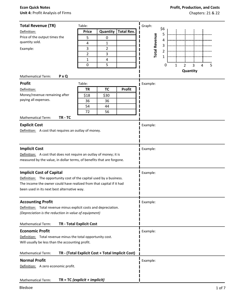
Econ Quick Notes
Unit 4: Profit Analysis of Firms
Table:
Definition:
Price of the output times the
quantity sold.
Example:
Mathematical Term:
Quantity Total Rev.
0
1
2
3
4
5
$6
5
4
3
2
1
0
1
2
3
4
Quantity
5
PxQ
Profit
Table:
Definition:
Money/revenue remaining after
paying all expenses.
Mathematical Term:
Price
5
4
3
2
1
0
Graph:
Total Revenue
Total Revenue (TR)
Profit, Production, and Costs
Chapters: 21 & 22
TR
$18
36
54
72
Example:
TC
$30
36
44
56
Profit
TR - TC
Explicit Cost
Example:
Definition: A cost that requires an outlay of money.
Implicit Cost
Example:
Definition: A cost that does not require an outlay of money; it is
measured by the value, in dollar terms, of benefits that are forgone.
Implicit Cost of Capital
Example:
Definition: The opportunity cost of the capital used by a business.
The income the owner could have realized from that capital if it had
been used in its next best alternative way.
Accounting Profit
Example:
Definition: Total revenue minus explicit costs and depreciation.
(Depreciation is the reduction in value of equipment)
Mathematical Term:
TR - Total Explicit Cost
Economic Profit
Example:
Definition: Total revenue minus the total opportunity cost.
Will usually be less than the accounting profit.
Mathematical Term:
TR - (Total Explicit Cost + Total Implicit Cost)
Normal Profit
Example:
Definition: A zero economic profit.
Mathematical Term:
Bledsoe
TR = TC (explicit + implicit)
1 of 7
Econ Quick Notes
Unit 4: Profit Analysis of Firms
Definition:
The change in total revenue
generated by an additional unit of
output.
TR
MR
0
2
4
6
8
10
12
14
$0
36
72
108
144
180
216
252
-
4
6
Q
8
10
12
14
Graph:
Q
TC
MC
0
2
4
6
8
10
12
14
$28
60
72
88
112
144
184
232
-
$28
24
20
16
12
8
4
0
2
4
6
8
10
12
14
Q
The marginal cost curve shows how the cost of producing one
more unit depends on the quantity that has already been
produced.
∆TC / ∆Q
Graph: (Draw both curves)
Optimal Output Rule
Explanation: Profit is maximized by producing the quantity of output at
which the marginal revenue of the last unit produced is equal to its
marginal cost.
Table: (Use the information from above tables to complete)
Principle of Marginal
Analysis : Every action
should continue until
marginal benefit equals
marginal cost.
2
The marginal revenue curve shows how marginal
revenue varies as output varies.
Table:
Definition:
The change in total cost generated
by an additional unit of output.
$28
24
20
16
12
8
4
0
∆TR / ∆Q
Marginal Cost (MC)
Mathematical Term:
Q
Graph:
Q
MR
MC
0
2
4
6
8
10
12
14
-
-
Profit
*Reminder : Profit = TR -TC, use tables above to
calculate.
●If MR > MC, then increasing production will increase profit.
●If MR < MC, then increasing production will decrease profit.
●If MR = MC, then profits are maximized.
Price, cost of unit
Mathematical Term:
Market Price is $18
Marginal Revenue
Table:
Marginal Cost
Marginal Revenue (MR)
Profit, Production, and Costs
Chapters: 21 & 22
$28
24
20
16
12
8
4
0
2
4
6 8 10
Quantity
12
14
Where the MR curve intersects the MC curve
determines the optimal output (maximizes profit)
for the firm.
Mathematical Term:
MR = MC
Bledsoe
2 of 7
Econ Quick Notes
Unit 4: Profit Analysis of Firms
Profit, Production, and Costs
Chapters: 21 & 22
Production Function
Example:
Definition: The relationship between the quantity of inputs a firm uses
and the quantity of output it produces.
*A firm's production function underlies its cost curves.
Fixed Input
Example:
Definition: An input whose quantity is fixed for a period of time and
cannot be varied.
Variable Input
Example:
Definition: An input whose quantity the firm can vary at any time.
Short Run
Example:
Definition: The time period in which at least one input is fixed.
Long Run
Example:
Definition: The time period in which all inputs can be varied.
Total Product (TP)
Graph:
Definition:
Total quantity, or total output, of a
good produced at each quantity of
labor employed.
Note:
The slope of TP is MP.
Mathematical Term:
Bledsoe
Table:
Labor
Q of carrots
(workers)
(bushels)
0
1
2
3
4
5
6
7
8
0
10
26
45
60
70
78
84
88
Total
Product
Q
90
80
70
60
50
40
30
20
10
0
The total product curve shows how the quantity
of output depends on the quantity of the variable
input, for a given quantity of the fixed input.
1
2
3
5
4
Labor
6
7
8
Q
3 of 7
Econ Quick Notes
Unit 4: Profit Analysis of Firms
Profit, Production, and Costs
Chapters: 21 & 22
Marginal Product (MP)
Definition:
Table:
The additional quantity of output
produced by using one more unit of an
input.
Graph:
MP
Q = TP
Labor
Q of carrots
Marginal
(workers)
(bushels)
Product
0
1
2
3
4
5
6
7
8
0
10
26
45
60
70
78
84
88
-
Note : Marginal Physical Product (MPP)
is the same thing as Marginal Product
(MP).
Example:
● If MP were to reach 0, then TP
would be at its peak.
20
18
16
14
12
10
8
6
4
2
0
1
2
3
Mathematical Term:
*MP is the slope of the TP curve
∆TP / ∆L
(L represents labor, however ∆I could be used for change in input.)
Diminishing Returns
5
4
Labor
6
7
8
Why does this happen?
Definition:
An increase in the quantity of an input, holding the levels of all other inputs
fixed, leads to a decline in the marginal product of that input.
Law of diminishing marginal productivity : In the short run, as variable
inputs are applied to fixed inputs, production first increases at an
increasing rate; then, production increases at a decreasing rate.
Average Product (AP)
Definition:
Labor
Q of carrots
Average
(workers)
(bushels)
Product
0
1
2
3
4
5
6
7
8
0
10
26
45
60
70
78
84
88
-
Relationship between marginal and
average curves:
●If marginal > avg, the avg is rising
●If marginal < avg, the avg is falling
Mathematical Term:
Graph:
AP/MP
Table:
A measure of average
labor productivity. Total
product divided by the
amount of labor employed.
On the above graph when do diminishing
marginal returns begin?
20
18
16
14
12
10
8
6
4
2
0
MP
1
2
3
5
4
Labor
6
7
8
Q / L or TP / # of inputs
Relationship between MP and MC
(Explains shape of MC curve)
●If marginal product is rising, marginal cost is falling
●If marginal product is falling, marginal cost is rising
*Simply because MP is declining (diminishing returns) and MC is rising does
not necessarily mean the firm should discontinue production.
Graph:
Q
$
MC
MP
Why?
Quantity of Labor
Bledsoe
Quantity of Output
4 of 7
Econ Quick Notes
Unit 4: Profit Analysis of Firms
Profit, Production, and Costs
Chapters: 21 & 22
Fixed Cost (FC)
Example:
Imagine setting up a successful lemonade stand on
your street corner. You are able to sell 1,000 cups a
month for $1 each. You have to rent a table from
your parents for $75 a month, lemons, sugar and
cups cost you $300 a month, and a monthly vendor’s
license cost $25 a month..
Definition: A cost that does not depend on the quantity of output
produced. It is the cost of the fixed input.
Total Fixed Cost (TFC) = Sum of all fixed costs.
Variable Cost (VC)
Definition: A cost that depends on the quantity of output produced. It
is the cost of the variable input.
Revenue Fixed Cost Var. Cost Total Cost Profit
P=
1.)
Q=
2.)
1.)
TFC=
TR=
TVC=
TC =
Total Variable Cost (TVC) = Sum of all variable costs.
Total Cost (TC)
Graph: Use the cost table below
Definition: The total cost of producing a given quantity of output is the
sum of the fixed cost and the variable cost of producing that quantity
of output.
TFC + TVC
Total Cost
Mathematical Term:
Complete the table using the following information:
● Renting the equipment costs $400
● Each worker must be paid $200
Output
Variable Cost
Fixed Cost
Total Cost
L
0
1
2
3
4
5
6
7
8
Q
0
18
40
55
65
73
78
80
81
VC
FC
TC
Definition:
Total cost divided by
quantity of output
produced.
Mathematical Term:
Bledsoe
Table: (Use the information from
above tables to complete)
Average Total Cost (ATC)
TC / Q
Note:
Change in
total cost
is reflected
dollar for
dollar in
change in
variable
costs.
Output
Total Cost
Avg Total Cost
Q
0
18
40
55
65
73
78
80
81
TC
ATC
-
or
AFC + AVC
0
20
40 60 80
Output (Q)
100
The total cost curve shows how total cost
depends on the quantity of output.
Graph: Use the cost table to the left
Average Total Cost
Q of Labor
$2,000
1,800
1,600
1,400
1,200
1,000
800
600
400
200
$32
30
28
26
24
22
20
18
16
15
30
45
60
Q
75 90
5 of 7
Econ Quick Notes
Unit 4: Profit Analysis of Firms
Definition:
The fixed cost per unit
of output.
Avg Fixed Cost
Q
0
18
40
55
65
73
78
80
81
FC
400
400
400
400
400
400
400
400
400
AFC
-
Output
Variable Cost
Q
0
18
40
55
65
73
78
80
81
VC
0
200
400
600
800
1000
1200
1400
1600
Graph: Use the cost table to the left
$24
21
18
15
12
9
6
3
15
TFC / Q
Average Variable Cost (AVC)
Definition:
The variable cost per
unit of output.
Mathematical Term:
Fixed Cost
Avg Variable
Cost
AVC
-
30 45 60
Output (Q)
75 90
Graph: Use the cost table to the left
Average Variable Cost
Mathematical Term:
Output
Average Fixed Cost
Average Fixed Cost (AFC)
Profit, Production, and Costs
Chapters: 21 & 22
$24
21
18
15
12
9
6
3
15
TVC / Q
30 45 60
Output (Q)
75 90
Explaining the U-shaped Average Total Cost Curve
ATC
● Spreading effect: The larger the output, the greater the quantity of output
● Diminishing returns effect: The larger the output, the greater amount of
Cost
over which fixed cost is spread, leading to lower average fixed cost.
variable inputs required to produce additional units, leading to higher
average variable cost.
Output (Q)
Definition:
The quantity of output at which average total cost is lowest. It
corresponds to the bottom of the U-shaped average total cost curve.
Relationship between marginal and
average curves:
●If marginal < avg, the avg is falling
●If marginal > avg, the avg is rising
Graph:
MC
ATC
Cost
Minimum-cost Output / Minimum Efficient Scale
Minimum-cost Output
Output (Q)
Bledsoe
6 of 7
Econ Quick Notes
Unit 4: Behind the Supply Curve: Profit, Production, and Costs
Graph:
LRATC
Cost
Long-Run Average Total Cost Curve (LRATC)
Definition: Shows the relationship between output and average total
cost when fixed cost has been chosen to minimize average total cost for
each level of output.
Note: Each Short-run Average Total Cost Curve (SRATC) represents a fixed
cost that can be chosen.
Profit, Production, and Costs
Chapters: 21 & 22
Example:
Output (Q)
Economies of Scale / Increasing Returns to Scale
Graph:
Economies of scale can result from increasing returns to scale, which exist
when output increases more than in proportion to an increase in all inputs
(doubling the inputs would more than double the output).
Cost
Definition: When long-run average total cost declines as output
increases.
Example:
Output (Q)
Constant Returns to Scale
Graph:
Example:
Cost
Definition: When output increases directly in proportion to an increase
in all inputs (doubling the inputs results in doubling the outputs).
Output (Q)
Diseconomies of Scale / Decreasing Returns to Scale
Graph:
Diseconomies of scale can result from decreasing returns to scale, which
exist when output increases less than in proportion to an increase in all
inputs (doubling the inputs would result in less than double the output).
Cost
Definition: When long-run average total cost increases as output
increases.
Example:
Output (Q)
Sunk Cost
Example:
Definition: A cost that has already been incurred and is nonrecoverable.
A sunk cost should be ignored in a decision about future actions.
Bledsoe
7 of 7