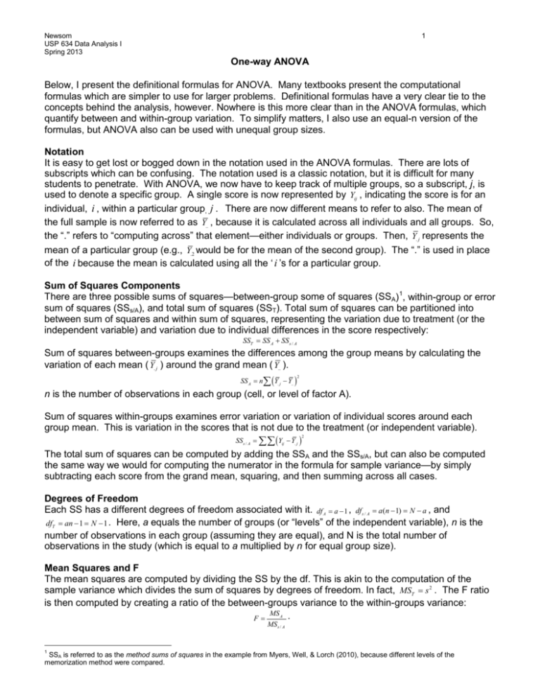
Newsom
USP 634 Data Analysis I
Spring 2013
1
One-way ANOVA
Below, I present the definitional formulas for ANOVA. Many textbooks present the computational
formulas which are simpler to use for larger problems. Definitional formulas have a very clear tie to the
concepts behind the analysis, however. Nowhere is this more clear than in the ANOVA formulas, which
quantify between and within-group variation. To simplify matters, I also use an equal-n version of the
formulas, but ANOVA also can be used with unequal group sizes.
Notation
It is easy to get lost or bogged down in the notation used in the ANOVA formulas. There are lots of
subscripts which can be confusing. The notation used is a classic notation, but it is difficult for many
students to penetrate. With ANOVA, we now have to keep track of multiple groups, so a subscript, j, is
used to denote a specific group. A single score is now represented by Yij , indicating the score is for an
individual, i , within a particular group, j . There are now different means to refer to also. The mean of
the full sample is now referred to as Y.. , because it is calculated across all individuals and all groups. So,
the “.” refers to “computing across” that element—either individuals or groups. Then, Y. j represents the
mean of a particular group (e.g., Y.2 would be for the mean of the second group). The “.” is used in place
of the i because the mean is calculated using all the ‘ i ’s for a particular group.
Sum of Squares Components
There are three possible sums of squares—between-group some of squares (SSA) 1, within-group or error
sum of squares (SSs/A), and total sum of squares (SST). Total sum of squares can be partitioned into
between sum of squares and within sum of squares, representing the variation due to treatment (or the
independent variable) and variation due to individual differences in the score respectively:
SS
=
SS A + SS s / A
T
Sum of squares between-groups examines the differences among the group means by calculating the
variation of each mean ( Y. j ) around the grand mean ( Y.. ).
=
SS A n∑ (Y. j − Y.. )
2
n is the number of observations in each group (cell, or level of factor A).
Sum of squares within-groups examines error variation or variation of individual scores around each
group mean. This is variation in the scores that is not due to the treatment (or independent variable).
=
SS s / A
∑∑ (Y
ij
− Y. j )
2
The total sum of squares can be computed by adding the SSA and the SSs/A, but can also be computed
the same way we would for computing the numerator in the formula for sample variance—by simply
subtracting each score from the grand mean, squaring, and then summing across all cases.
Degrees of Freedom
Each SS has a different degrees of freedom associated with it. df A= a − 1 , df s / A = a(n − 1) = N − a , and
dfT = an − 1 = N − 1 . Here, a equals the number of groups (or “levels” of the independent variable), n is the
number of observations in each group (assuming they are equal), and N is the total number of
observations in the study (which is equal to a multiplied by n for equal group size).
Mean Squares and F
The mean squares are computed by dividing the SS by the df. This is akin to the computation of the
sample variance which divides the sum of squares by degrees of freedom. In fact, MST = s 2 . The F ratio
is then computed by creating a ratio of the between-groups variance to the within-groups variance:
MS A .
F=
MS s / A
1
SSA is referred to as the method sums of squares in the example from Myers, Well, & Lorch (2010), because different levels of the
memorization method were compared.
Newsom
USP 634 Data Analysis I
Spring 2013
2
Example of a Three-group ANOVA
The following is a hypothetical example comparing satisfaction ratings of teachers randomly assigned to public, charter, and private
schools (e.g., Catholic schools).
Public
(Y
ij
4
4
6
8
8
− Y.1 )
4
4
0
4
4
Y.1 = 6
∑ (Y
(Y
2
ij
− Y.1 ) =
16
− Y.. )
2
9
9
1
1
1
2
ij
(Y
Charter
ij
9
8
10
8
10
− Y.2 )
0
1
1
1
1
∑ (Y
Y.2 = 9
ij
(Y
2
ij
− Y.2 ) =
4
− Y.. )
4
1
9
1
9
2
Private
ij
6
6
6
7
5
Y.3 = 6
2
(Y
− Y.3 )
0
0
0
1
1
∑ (Y
ij
(Y
2
ij
− Y.. )
2
1
1
1
0
4
− Y.3 ) =
2
2
Y.. = 7
ANOVA Table
2
2
2
SS A = n∑ (Y. j − Y.. ) = 5 ( 6 − 7 ) + ( 9 − 7 ) + ( 6 − 7 )  = 30


2
SS s / A =
SST =
∑∑ (Y
ij
∑ (Y
ij
− Y. j ) = 16 + 4 + 2 = 22
2
df = a − 1 = 3 − 1 = 2
df = N − a = 15 − 3 = 12
SS A 30
MS A
15
=
F
= = 8.182
= = 15
MS s / A 1.83
df A
2
SS s / A 22
MS s=
= = 1.833
/A
df s / A 12
MS=
A
− Y.. ) = 52
2
Fcrit with df of 2 and 12 is 3.88, so the calculated F is significant.
An analysis of variance tested whether there were differences in satisfaction among public, charter, and private school teachers. Charter
school teachers had higher satisfaction ratings (M = 9) compared to public and private school teachers (both M = 6). Results indicated that
these means differed significantly, F(2,12) = 8.18, p < .01. The proportion of variance in satisfaction accounted for by type of school was
approximately 58% (η2 = .58)
One can then estimate the magnitude of the effect of the independent variable by computing η 2 or ω 2 :
2
η=
SS A 30
= = .58 or 58%
SST 52
=
ω2
SS A − ( a − 1)( MS s / A ) 30 − ( 3 − 1)1.83
= = .49 or 49%
SST + MS s / A
52 + 1.83