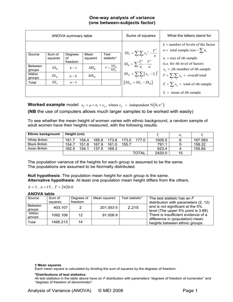
One-way analysis of variance
(one between-subjects factor)
Sums of squares
ANOVA summary table
What the letters stand for
k = number of levels of the factor
Source
Between
groups
Within
groups
Total
Sum of
squares
Degrees
of
freedom
Mean
square†
SSB
k −1
MSB
SS W
n−k
MS W
SST
n −1
SST = ∑∑ xij 2 −
Test
statistic*
F=
i
SS B = ∑
MS B
MS W
i
j
i
ni = size of ith sample
Ti 2 T 2
−
ni
n
SSW = ∑∑ ( xij − xi )
i
n = total sample size = ∑ ni
T2
n
j
[ SSW = SST − SSB ]
2
(i.e. for ith level of factor)
xij = jth member of ith sample
T = ∑∑ xij = overall total
i
j
Ti = ∑ xij = total of ith sample
j
xi = mean of ith sample
Worked example model: xij = μ + αi + εij , where εij ∼ independent N ( 0, σ 2 )
(NB the use of computers allows much larger samples to be worked with easily)
To see whether the mean height of women varies with ethnic background, a random sample of
adult women have their heights measured, with the following results.
Ethnic background
Height (cm)
White British
Black British
Asian British
161.7
154.7
162.5
154.4
151.8
154.1
165.8
167.9
137.5
173.6
161.0
169.3
173.0
155.7
177.0
TOTAL
Ti
1005.5
791.1
623.4
2420.0
xi
ni
6
5
4
15
167.583
158.22
155.85
The population variance of the heights for each group is assumed to be the same.
The populations are assumed to be Normally distributed.
Null hypothesis: The population mean height for each group is the same.
Alternative hypothesis: At least one population mean height differs from the others.
k = 3 , n = 15 , T = 2420.0
ANOVA table
Source
Between
groups
Within
groups
Total
Sum of
squares
Degrees of
freedom
Mean square†
403.107
2
201.553 5
1092.106
12
91.008 9
1495.213
14
Test statistic*
2.215
The test statistic has an F
distribution with parameters (2, 12)
and is not significant at the 5%
level (The upper 5% point is 3.89).
There is insufficient evidence of a
difference in (population) mean
heights between ethnic groups.
† Mean squares
Each mean square is calculated by dividing the sum of squares by the degrees of freedom.
*Distributions of test statistics
All test statistics in the table above have an F distribution with parameters “degrees of freedom of numerator” and
“degrees of freedom of denominator”.
Analysis of Variance (ANOVA)
© MEI 2008
Page 1
Two-way analysis of variance
(no interaction)
ANOVA summary table
Source
Sum of
squares
Degrees of
freedom
b −1
SSB
Factor B
SSR
Residual
n − a − b +1
SST = ∑∑∑ xijk
Test
statistic*
MSA
MSA
F=
MS R
MSB
MS B
F=
MSR
i
j
k
2
SSB = ∑
j
What the letters stand for
a = number of levels of factor A
T 2 b = number of levels of factor B
−
n r = number of data values for each
T2 T2
SSA = ∑ i −
n
i rb
MSR
(by
subtraction)
Tj2
T2
−
ra n
combination of levels of A and B
n = rab = total sample size
xijk = kth member of sample at
level i of factor A & level j of factor B
T = ∑∑∑ xijk = overall total
i
j
k
SSR = SST − ( SS A + SSB ) Ti =
total of data
at level i of factor A
Tj =
total of data
at level j of factor B
n −1
SST
Total
Mean
square†
a −1
SSA
Factor A
Sums of squares
Worked example model: xij = μ + αi + β j + εij , where εij ∼ independent N ( 0, σ 2 )
(NB the use of computers allows much larger samples to be worked with easily)
Two laboratories test the calorific content of four brands of digestive biscuit. Three of each variety of biscuit
are tested by each laboratory with the following results. The number of calories per biscuit is shown.
Lab 1
Biscuit I
Biscuit II
Biscuit III
Biscuit IV
73.6
69.3
75.8
71.1
Tj
72.2
67.6
75.7
66.7
74.3
70.1
76.4
69.8
862.6
Ti
Lab 2
70.9
70.6
72.5
70.5
73.7
69.6
73.0
71.2
75.5
69.9
71.6
70.4
859.4
440.2
417.1
445.0
419.7
T = 1722
The population variance of the number of calories per biscuit is assumed to be the same for each
combination of laboratory and biscuit brand. It is assumed that there is no interaction between the factors
(see page 5 for “with interaction”). The populations are assumed to be Normally distributed.
Null hypotheses: (a) The population mean number of calories per biscuit is the same for each brand.
(b) The population mean number of calories per biscuit is the same for each of the laboratories.
Alternative hypotheses: (a) At least one population mean calorie count differs from the other brands.
(b) At least one population mean calorie count differs from the other laboratories.
Factor A is biscuit brand. Factor B is laboratory. a = 4, b = 2, r = 3, n = 24
ANOVA table
Source
Factor A
Factor B
Residual
Total
Sum of
Degrees of
squares
freedom
100.09
3
0.4267
1
52.703
19
153.22
23
Mean
square†
33.363
0.4267
2.774
Test
statistic*
12.03
0.154
The critical value for F3,19 at the 5% level is 3.13.
12.03 is bigger than this so there is evidence that
not all brands of biscuit have the same population
mean calorie count.
The critical value for F1,19 at the 5% level is 4.38. 0.137 is less than this so there is no evidence of a
difference between laboratories in respect of the population mean calorie count.
† Mean squares
Each mean square is calculated by dividing the sum of squares by the degrees of freedom.
*Distributions of test statistics
All test statistics in the table above have an F distribution with parameters “degrees of freedom of numerator” and
“degrees of freedom of denominator”.
Analysis of Variance (ANOVA)
© MEI 2008
Page 2
Analysis of variance for randomised blocks
ANOVA summary table
Source
Sum of
squares
Factor A
(treatment)
Factor B
(blocks)
Degrees of
freedom
Mean
square
†
a −1
SSA
b −1
SSB
n − a − b +1
Residual
SSR
(by
subtraction)
Total
SST
n −1
Sums of squares
Test
statistic*
MSA
MS R
MSA
F=
MSB
MS B
F=
MSR
SST = ∑∑∑ xijk 2 −
i
k
SSA = ∑
Ti T 2
−
rb n
SSB = ∑
Tj
i
j
MSR
j
What the letters stand for
T
n
2
2
2
ra
−
T2
n
SSR = SST − ( SS A + SSB )
a = number of levels of factor A
b = number of levels of factor B
r = number of data values for each
combination of levels of A and B
n = rab = total sample size
xijk = kth member of sample at
level i of factor A & level j of factor B
T = ∑∑∑ xijk = overall total
i
j
k
Ti =
total of data
at level i of factor A
Tj =
total of data
at level j of factor B
Worked example model: xij = μ + αi + β j + εij , where εij ∼ independent N ( 0, σ 2 )
(NB the use of computers allows much larger samples to be worked with easily)
Four varieties of garden pea (C, D, E and F) are planted in a randomised block design in strips in a field
which has a stream flowing down one side. The treatment factor is pea variety. The blocking (nuisance)
factor is distance from the stream. The mean yield per plant (grammes) is shown in the table below.
Pea C
Pea D
Pea E
Pea F
Tj
Strip 1
Strip 2
Strip 3
294
324
322
263
1203
274
335
278
280
1167
305
256
286
285
1132
Ti
873
915
886
828
T =3502
The population variance of the mean yield is assumed to be the same for each combination of variety and
strip. It is assumed that there is no interaction between the factors. The populations are assumed to be
Normally distributed. a = 4, b = 3, r = 1, n = 12 .
Null hypotheses: (a) The population mean yield is the same for each pea variety.
(b) The population mean yield is the same for each strip.
Alternative hypotheses: (a) At least one population mean yield for a variety differs from the other varieties.
(b) At least one population mean yield for a strip differs from the other strips.
ANOVA table
Source
Variety
Strips
Residual
Total
Sum of
Degrees of
squares
freedom
1311
3
630.17
2
4980.5
6
6831.7
Mean
square†
437
315.08
830.08
Test
statistic*
0.526
0.3796
The critical value for F3,11 at the 5% level is 3.59.
0.526 is less than this so there is no evidence of
a difference in population mean yield between
pea varieties.
11
The critical value for F2,11 at the 5% level is 3.98. 0.3796 is less than this so there is no evidence of a
difference between strips in respect of population mean yield.
† Mean squares
Each mean square is calculated by dividing the sum of squares by the degrees of freedom.
*Distributions of test statistics
All test statistics in the table above have an F distribution with parameters “degrees of freedom of numerator” and
“degrees of freedom of denominator”.
Analysis of Variance (ANOVA)
© MEI 2008
Page 3
Analysis of variance for Latin square
ANOVA summary table
Source
Sum of
squares
Degrees of
freedom
Mean
square†
Sums of squares
Test
statistic*
MS rows
F=
MS R
Rows
SS rows
n −1
MS rows
Columns
SScols
n −1
MScols
F=
MScols
MS R
Treatments
SS treats
n −1
MS treats
F=
MS treats
MSR
Residual
SSR
Total
SST
(n − 1)(n − 2)
MSR
(by
subtraction)
T2
SST = ∑∑ xij − 2
n
i
j
2
SSrows = ∑
Tr T
−
n n2
SScols = ∑
Tc T
−
n n2
r
c
2
2
What the letters stand for
n = number of rows (or columns)
xij = observation in
row i and column j
2
T = ∑∑ xij = overall total
i
2
j
Tr = total of data in row r
Tk 2 T 2
Tc = total of data in column c
−
n n2
k
total of data at
SSR = SST − ( SSrows + SScols + SS treats ) Tk =
one level of the treatment
SStreats = ∑
n2 − 1
Worked example model: xij ( k ) = μ + αi + β j + γk + εij ( k ) , where εij ( k ) ∼ independent N ( 0, σ 2 )
An experiment to test whether four varieties of potato give the same mean yield is carried out in a square
field subdivided into a square grid of plots of equal size. It is thought that the field might have natural “fertility
gradients” both across and down it. To allow for this possibility, a Latin square design is used. The table
shows the layout of the field and the yield in kg per plot. The rows and columns represent the possible
fertility gradients (these are nuisance factors). The letters A, B, C, D represent the varieties of potato (the
factor of interest). n = 4.
A
D
B
C
Col Total
19.8
21.3
20.8
20.4
82.3
B
A
C
D
21.2
21.0
18.3
16.1
76.6
D
C
A
B
22.0
18.8
20.7
18.4
79.9
C
B
D
A
18.6
18.7
17.1
14.3
68.7
Row Total
81.6
79.8
76.9
69.2
307.5
Variety
A
B
C
D
Total
Total
75.8
79.1
76.1
76.5
307.5
Null hypotheses:
(a) The population mean yield is the same for all varieties.
(b) The population mean yield is the same in each row (i.e. no fertility gradient in this direction).
(c) The population mean yield is the same in each column (i.e. no fertility gradient in this direction)
Alternative hypotheses: Each null hypothesis has a corresponding alternative hypothesis that at least one
population mean yield differs from the others
ANOVA table
Source
Rows
Columns
Treatments
(varieties)
Residual
Total
Sum of
Degrees of
squares
freedom
22.447
3
26.372
3
Mean
square†
7.482
8.791
1.712
3
0.571
15.814
6
2.636
66.344
15
Test
statistic*
2.839
3.335
0.217
The critical value for
F3,6 at the 5% level is 4.76.
2.839 and 3.335 are each smaller than 4.76 so there
is no evidence of a significant difference in mean
yields between rows or columns
0.217 is also smaller than 4.76 so there is no
evidence of difference in mean yield between
varieties.
NOTE The Latin square is also useful for situations where there are two “real-interest” factors and one
“nuisance” or three “real-interest” factors, provided all factors have the same number of levels and there is no
interaction. Simply use the rows and/or columns to represent the additional real-interest factor(s).
† Mean squares
Each mean square is calculated by dividing the sum of squares by the degrees of freedom.
*Distributions of test statistics
All test statistics in the table above have an F distribution with parameters “degrees of freedom of numerator” and
“degrees of freedom of denominator”.
Analysis of Variance (ANOVA)
© MEI 2008
Page 4
Two-way analysis of variance (with interaction)
(two between-subjects factors)
ANOVA summary table
Sums of squares
What the letters stand for
a = number of levels of factor A
b = number of levels of factor B
n = total sample size
Source
Sum of
squares
Degrees of
freedom
Mean
square
†
Test
statistic*
Factor A
SSA
a −1
MSA
MSA
F=
MS R
Factor B
SSB
b −1
MSB
F=
MS B
MSR
A×B
interaction
SSAB
MS AB
F=
MS AB
MS R
Residual
SSR
(by
subtraction)
Total
SST
n −1
(a − 1)(b − 1)
n − ab
MSR
SST = ∑∑∑ xijk
i
SSA = ∑
j
k
2
T2
−
n
Ti 2 T 2
−
ni
n
xijk = kth member of sample at
level i of factor A & level j of factor B
T = ∑∑∑ xijk = overall total
i
j
k
Ti =
total of data
at level i of factor A
Tj 2 T 2
SSB = ∑
−
ni = number of data items
n
j nj
at level i of factor A
Tg 2 T 2
Tj =
total of data
SSG = ∑
−
at
level
j of factor B
n
g ng
n
=
number
of data items
j
SSAB = SSG − ( SSA + SSB )
at level j of factor B
SS R = SS T − ( SS A + SS B + SS AB )
Tg = total of all the data at a particular level
i
of A and of B
(there are ab such groups)
ng = number of data values at a particular
level of A and of B
Worked example model: xijk = μ + αi + β j + γij + εijk , where εijk ∼ independent N ( 0, σ 2 )
(NB the use of computers allows much larger samples to be worked with easily)
In an experiment to test whether students achieve similar marks on computer based tests to those
they achieve on paper based tests, a random sample of students from three classes sit either a
paper based or a computer based test (the questions on both tests are the same). The marks they
achieve are shown:
Class
Class 2
Class 1
Computer
Test mode
Paper
Class totals
33
38
61
69
Total 201
53
47
36
47
Total 183
384
62
57
63
41
Total 223
37
42
45
52
Total 176
399
Class 3
62
44
39
45
Total 190
30
42
27
35
Total 134
324
Test mode
totals
614
493
1107
The variance for each section of the population is assumed to be the same. The population is
assumed normal.
Factor A is “test mode”; this is the factor of interest. Factor B is “class”; this is a nuisance factor.
a = 2, b = 3, n = 24, ni = 12 (all i ), n j = 8 (all j ), ng = 4 (all g ) .
See next page for ANOVA table and conclusion.
† Mean squares
Each mean square is calculated by dividing the sum of squares by the degrees of freedom.
*Distributions of test statistics
All test statistics in the table above have an F distribution with parameters “degrees of freedom of numerator” and
“degrees of freedom of denominator”.
Analysis of Variance (ANOVA)
© MEI 2008
Page 5
ANOVA table for two-way analysis of variance (two between-subjects factors)
Null hypotheses: (a) The population mean test mark is the same for either mode of test (paper or
computer).
(b) The population mean test mark is the same for each of the classes
(c) There is no interaction between test mode and class in respect of the population mean test
mark.
Alternative hypothesis: (a) The population mean test marks differ for the test modes.
(b) At least one population mean test mark differs from the other classes.
(c) There is some interaction between test mode and class in respect of the population mean test
mark.
Source
Sum of
squares
Degrees of
freedom
Mean
square†
Test statistic*
Distribution of
test statistic
Critical value at 5% level
Test mode
610.04
1
610.04
5.706
F1,18
4.41
Class
393.75
2
196.875
1.842
F2,18
3.55
0.461
F2,18
3.55
A×B
interaction
Residual
Total
98.585
2
1924.25
3026.625
18
23
49.2925
106.903
SSG = 1102.375
5.706 > 4.41 so there is evidence that there is a difference in the mean marks for different modes
of test.
1.842 < 3.55 so there is no evidence of difference in mean marks between the classes.
0.461 < 3.55 so there is no evidence of interaction between class and mode of test.
† Mean squares
Each mean square is calculated by dividing the sum of squares by the degrees of freedom.
*Distributions of test statistics
All test statistics in the table above have an F distribution with parameters “degrees of freedom of numerator” and
“degrees of freedom of denominator”.
Analysis of Variance (ANOVA)
© MEI 2008
Page 6
Kruskal-Wallis one-way analysis of variance
Calculation of test statistic
Rank all data values, sum the ranks for each group and
square these values.
Test statistic, H, is:
2
12 ⎛ R j
H=
⎜∑
N ( N + 1) ⎜⎝ N j
Distribution of test
statistic
What the letters stand for
⎞
⎟⎟ − 3( N + 1)
⎠
N j = size of sample j , N = ∑ N j ,
χ K2 −1
R j = sum of ranks for sample j
K = number of groups
Worked example
(NB the use of computers allows much larger samples to be worked with easily)
An investigation compares customer waiting times in three branches of a bank. The queuing
time of a random sample of customers in each branch is measured with the following results
(in minutes).
Branch
A
B
C
Waiting times (mins)
0
0
2.9
7.3
0.9
0.7
8.4
4.4
0.8
8.2
2.4
7.0
0
4.0
0.3
6.0
Null hypothesis: The mean waiting times for all three branches are the same.
Alternative hypothesis: The mean waiting times for all three branches are not the same.
Ranks in bold
Branch
Waiting times (mins)
0
2
7.3 14
8.4 16
A
B
C
N = 16,
0
2
0.9 7
4.4 11
2.9 9
0.7 5
0.8 6
8.2 15
2.4 8
7.0 13
0
2
4.0 10
0.3 4
6.0 12
Sum of ranks
( Rj )
Size of sample
( Nj )
42
44
50
6
5
5
K =3
⎞
⎟⎟ − 3( N + 1)
⎠
2
12 ⎛ 42
442 502 ⎞
H=
+
+
⎜
⎟ − 3 × 17
16 × 17 ⎝ 6
5
5 ⎠
H ≈ 1.1118
H=
2
12 ⎛ R j
⎜⎜ ∑
N ( N + 1) ⎝ N j
The 5% critical value for χ 22 is 5.991.
1.1118 < 5.991 so there is insufficient evidence, at the 5% level, that there is any difference in
mean waiting times between the three branches.
Analysis of Variance (ANOVA)
Page 7
Friedman’s two-way analysis of variance by rank
Calculation of test statistic
N = size of each sample (number of data
items in each column),
K = number of samples (number of data
items in each row),
Put the data in a table. To test whether there is a
significant difference between the sets of data in the
columns, rank each row and sum the ranks for each
column.
Test statistic, M, is:
M=
Distribution of test
statistic
What the letters stand for
Ri = sum of ranks for sample i
K
12
∑ Ri2 − 3N ( K + 1)
NK ( K + 1) i =1
χ K2 −1
(sum of ranks of column i )
Worked example
Five judges give a mark out of 15 to each of three paintings. Is there a significant difference
between the judges?
Judge
Painting
sunset 1
sunset 2
sunrise
A
B
C
D
E
7
9
13
5
8
13
8
10
14
6
8
13
9
11
13
Null hypothesis: There is no significant difference between the judges.
Alternative hypothesis: There is a significant difference between the judges.
The factor of interest is whether the judges agree. The “nuisance” factor is “painting”.
Ranking the rows
Judge
Painting
sunset 1
sunset 2
sunrise
rank sum
A
7
9
13
3
3
2.5
8.5
B
5 1
8 1.5
13 2.5
5
C
8
10
14
4
4
5
13
D
6 2
8 1.5
13 2.5
6
E
9
11
13
5
5
2.5
12.5
N = 3, K = 5
K
12
M=
∑ Ri2 − 3N ( K + 1)
NK ( K + 1) i =1
12
M=
( 8.52 + 52 + 132 + 62 + 12.52 ) − 3 × 3 × 6
3× 5 × 6
M = 7.13
The critical value at the 5% level for χ 42 is 9.488.
7.13 < 9.488 so there is insufficient evidence of a significant difference in the marks given by
the five judges.
Analysis of Variance (ANOVA)
Page 8