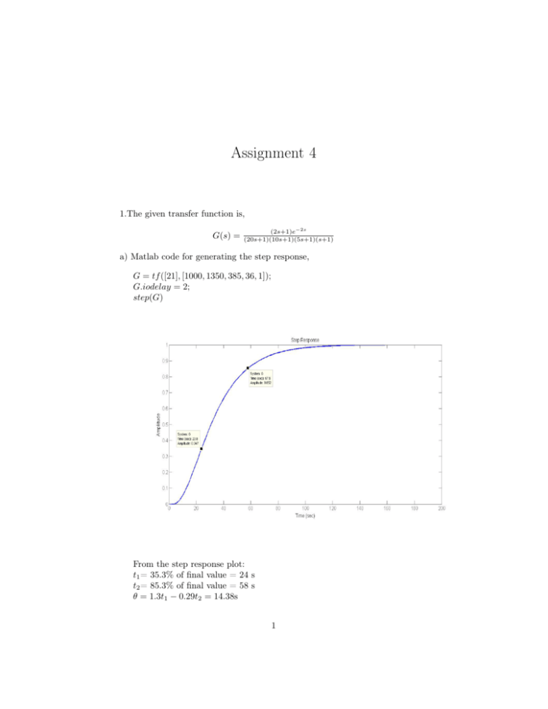
Assignment 4
1.The given transfer function is,
G(s) =
(2s+1)e−2s
(20s+1)(10s+1)(5s+1)(s+1)
a) Matlab code for generating the step response,
G = tf ([21], [1000, 1350, 385, 36, 1]);
G.iodelay = 2;
step(G)
From the step response plot:
t1 = 35.3% of final value = 24 s
t2 = 85.3% of final value = 58 s
θ = 1.3t1 − 0.29t2 = 14.38s
1
τ = 0.67(t2 − t1 ) = 22.78s
The FOPTD model using Krishnaswamy & Sundaresan’s method is given
by,
G(s) =
Ke−θs
τ s+1
=
e−14.38s
22.78s+1
b) Skogestad’s half rule method
FOPTD approximation:
1
θ = 2 + 10
2 + 5 + 1 − 2 = 12.5
10
τ = 20 + 2 = 25
The approximate FOPTD model is given by,
G(s) =
Ke−θs
τ s+1
=
e−12.5s
25s+1
SOPTD approximation:
θ = 2 + 52 + 1 − 12 = 5
τ1 = 20; τ2 = 10 + 52 = 12.5
The approximate SOPTD model is given by,
G(s) =
Ke−θs
(τ1 s+1)(τ2 s+1)
=
e−5s
(20s+1)(12.5s+1)
c) The Matlab code is:
function G_ls = modpred(par,data)
K = par(1);
tau1 = par(2);
tau2 = par(3);
den = sqrt((1+(tau1*data).^2).*(1+(tau2*data).^2));
G_ls = K./den;
end
In the command window:
G1=zpk([-0.5],[-0.05,-0.1,-0.2,-1],0.002);
G1 =
0.002(s+0.5)
(s+0.5)(s+0.1)(s+0.2)(s+1)
[mag,phase,w] = bode(G_1);
par = lsqcurvefit(@(par,data)modpred(par,data),[1 1 1]’,w,squeeze(mag));
G_lsq = tf([par(1)],[par(2)*par(3) par(2)+par(3) 1]);
G_lsq.iodelay = 2;
Transfer function:
G_lsq =
0.9995e−2s
251.4s2 +31.7s+1
2
d) Comparison from the plots:
3
Properties
Settling Time
Rise Time
Delay
Time constant
Fit
G
98.7
53.3
2
38.2
-
G_ks
104
50.1
14.38
22.78
Good
G_sf
110
54.9
12.5
25
Worse
G_ss
102
55.3
5
12.5
Worst
2. a) The SIMULINK block diagram of the process G(s) =
ZOH discretization (Ts = 0.5s)
G_ls
94.5
53.3
2
36
Best
2e−0.5s
(5s+1)(s+2)
b) Matlab code for generating pseudo-random binary signal (PRBS):
u = idinput(1530,0 prbs0 , [0, 0.15]);
4
with
5
c) y[k] =
M
X
g[n]u[k − n]
n=0
6
M = 20
Matlab code:
for i = 20+1 : 1530
y_reg(i-20) = y.signals.values(i);
for n = 1:21
A(i-20,n) = u(i+1-n);
end
end
g = A\y_reg’;
The value of n at which the IR coefficient has a significant value for the first
time is the delay. Here d = 2.
d) y[k] = a1 y[k − 1] + a2 y[k − 2] + b1 u[k − d − 1] + b2 u[k − d − 2]
Matlab code:
for k = 5:1530
y_par(k-2-2) = y.signals.values(k);
A_par(k-2-2,1) = y.signals.values(k-1);
A_par(k-2-2,2) = y.signals.values(k-2);
A_par(k-2-2,3) = u(k-3);
A_par(k-2-2,4) = u(k-4);
end
parameters = A_par\y_par;
The parameters estimated using least square method:
a1 = 0.2954, a2 = 0.3504, b1 = 0.0848and b2 = 0.0982
y[k] = 0.2954y[k − 1] + 0.3504y[k − 2] + 0.0848u[k − 3] + 0.0982u[k − 4]
Y (z) = 0.2954z −1 Y (z) + 0.3504z −2 Y (z) + 0.0848z −3 U (z) + 0.0982z −4 U (z)
G(z) =
Y (z)
U (z)
=
0.0848z −3 +0.0982z −4
1−0.2954z −1 −0.3504z −2
=
0.0848z+0.0982
z 4 −0.2954z 3 −0.3504z 2
Comparison with the theoretical model, G(z) =
sumed model is not close.
3. Ga (s) = Kc
τD s+1
ατD s+1
0.0355z+0.02465
z 3 −1.273z 2 +0.3329z ,
Gi (s) = Kc (τD s + 1)
a) For step response: u(t) = A;U (s) =
A
s
Ya (s) = Ga (s).U (s) = Kc A
τD s+1
s(ατD s+1)
Taking inverse Laplace transform
−t
ya (t) =
Kc A ατD
α e
−t
+ Kc A(1 − e ατD )
When α → 0
7
the as-
ya (t) = Kc A(δ(t)τD + 1)
For ideal response,
Yi (s) = Kc AτD +
Kc A
s
Taking inverse Laplace transform
yi (t) = Kc A(δ(t)τD + 1)
When α → 0
yi (t) = Kc A(δ(t)τD + 1)
So,
ya (t) = yi (t) as α → 0
For ramp response:u(t) = At;U (s) =
A
s2
Ya (s) = Ga (s).U (s) = Kc A
= Kc AτD
h
1
s
−
ατD
ατD s+1
i
+ Kc A
h
τD s+1
s2 (ατD s+1)
−ατD
s
+
1
s2
+
(ατD )2
ατD s+1
i
Taking inverse Laplace transform
−t
−t
ya (t) = Kc AτD (1 − e ατD ) + Kc A(t − ατD (1 − e ατD ))
When α → 0
ya (t) = Kc A(τD + t)
For ideal response,
Yi (s) =
Kc AτD
s
+
Kc A
s2
Taking inverse Laplace transform
yi (t) = Kc A(τD + t)
So,
ya (t) = yi (t) as α → 0
b) It may be difficult to construct an analog device with this ideal transfer
function, it will require to find the exact derivative time τD to use in the
device. So it will be difficult to estimate accurately the derivative for use in
the ideal transfer function.
8
c) Derivative action is an anticipatory action. It will amplify the noise in the
measurement by taking its derivative. The approximate transfer function will
reduce this amplification by the approximation. So it is an advantage of not
being able to obtain ideal transfer function.
4. G(s) =
s2 +4s+8
s(s+1)(s+3) ;
a) GOL (s) =
H(s) =
1
s+10 ;
Gc (s) = Kc
Kc (s2 +4s+8)
s(s+1)(s+3)(s+10)
Poles: 0, −1,
P−3, −10
P and Zeros: −2 ± 2i So m-n=2
Centroid=
Pi −
Zi
m−n
= −5
Angle of asymptotes= 180+k(360)
= 900 , 2700 for k=0,1
m−n
Characteristic equation: 1 + Kc GOL (s) = 0
Kc = − s(s+1)(s+3)(s+10)
s2 +4s+8
To find break away point
dKc
ds
=0
i.e. s = −0.4969, −6.2868
Matlab code for the Root Locus plot:
num =[1 4 8];
den =[1 14 43 30 0];
G = tf (num, den);
rltool(G)
9
c)GCL (s) =
Kc (s2 +4s+8)
s(s+1)(s+3)(s+10)+KC (s2 +4s+8)
Poles of s(s + 1)(s + 3)(s + 10) + Kc (s2 + 4s + 8) = 0 by taking Kc = 1 will
be at s = −0.4969 ± 0.1128i, −3.1156 and −9.8906
10
At the damping of 0.4 the value of Kc = 27.3
Taking this value,
GCL (s) =
27.3s2 +98.2s+196.4
s(s+1)(s+3)(s+10)+27.3(s2 +4s+8)
11
From the Bode plot we can find the relative stability using phase margin.
d) For PI controller Gc (s) = Kc (1 +
GOL (s) =
1
τI s )
Kc (s2 +4s+8)(1+ τ 1 s )
I
s(s+1)(s+3)(s+10)
For tuning τI
The characteristic equation 1 + GOL = 0
1+
Kc (s2 +4s+8)(1+ τ 1 s )
I
s(s+1)(s+3)(s+10)
=0
τI =
−Kc (s2 +4s+8)
s2 (s+1)(s+3)(s+10)+Kc (s2 +4s+8)
Kc = −D(s)
N (s)
D(s) = Kc (s2 + 4s + 8)
N (s) = s5 + 14s4 + (Kc + 43)s3 + (30 + 4Kc )s2 + 8Kc
(s)
GOL (s) = N
D(s)
The effective open loop transfer function
GOL (s) =
s5 +14s4 +(Kc +43)s3 +(30+4Kc )s2 +8Kc
Kc (s2 +4s+8)
12