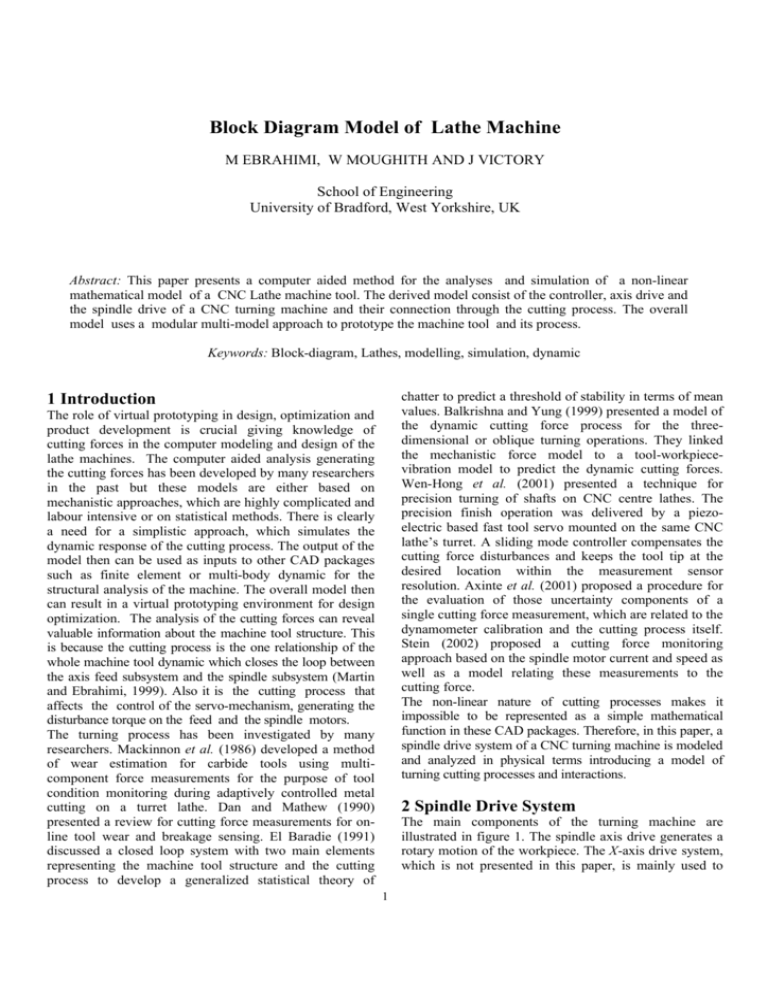
Block Diagram Model of Lathe Machine
M EBRAHIMI, W MOUGHITH AND J VICTORY
School of Engineering
University of Bradford, West Yorkshire, UK
Abstract: This paper presents a computer aided method for the analyses and simulation of a non-linear
mathematical model of a CNC Lathe machine tool. The derived model consist of the controller, axis drive and
the spindle drive of a CNC turning machine and their connection through the cutting process. The overall
model uses a modular multi-model approach to prototype the machine tool and its process.
Keywords: Block-diagram, Lathes, modelling, simulation, dynamic
chatter to predict a threshold of stability in terms of mean
values. Balkrishna and Yung (1999) presented a model of
the dynamic cutting force process for the threedimensional or oblique turning operations. They linked
the mechanistic force model to a tool-workpiecevibration model to predict the dynamic cutting forces.
Wen-Hong et al. (2001) presented a technique for
precision turning of shafts on CNC centre lathes. The
precision finish operation was delivered by a piezoelectric based fast tool servo mounted on the same CNC
lathe’s turret. A sliding mode controller compensates the
cutting force disturbances and keeps the tool tip at the
desired location within the measurement sensor
resolution. Axinte et al. (2001) proposed a procedure for
the evaluation of those uncertainty components of a
single cutting force measurement, which are related to the
dynamometer calibration and the cutting process itself.
Stein (2002) proposed a cutting force monitoring
approach based on the spindle motor current and speed as
well as a model relating these measurements to the
cutting force.
The non-linear nature of cutting processes makes it
impossible to be represented as a simple mathematical
function in these CAD packages. Therefore, in this paper, a
spindle drive system of a CNC turning machine is modeled
and analyzed in physical terms introducing a model of
turning cutting processes and interactions.
1 Introduction
The role of virtual prototyping in design, optimization and
product development is crucial giving knowledge of
cutting forces in the computer modeling and design of the
lathe machines. The computer aided analysis generating
the cutting forces has been developed by many researchers
in the past but these models are either based on
mechanistic approaches, which are highly complicated and
labour intensive or on statistical methods. There is clearly
a need for a simplistic approach, which simulates the
dynamic response of the cutting process. The output of the
model then can be used as inputs to other CAD packages
such as finite element or multi-body dynamic for the
structural analysis of the machine. The overall model then
can result in a virtual prototyping environment for design
optimization. The analysis of the cutting forces can reveal
valuable information about the machine tool structure. This
is because the cutting process is the one relationship of the
whole machine tool dynamic which closes the loop between
the axis feed subsystem and the spindle subsystem (Martin
and Ebrahimi, 1999). Also it is the cutting process that
affects the control of the servo-mechanism, generating the
disturbance torque on the feed and the spindle motors.
The turning process has been investigated by many
researchers. Mackinnon et al. (1986) developed a method
of wear estimation for carbide tools using multicomponent force measurements for the purpose of tool
condition monitoring during adaptively controlled metal
cutting on a turret lathe. Dan and Mathew (1990)
presented a review for cutting force measurements for online tool wear and breakage sensing. El Baradie (1991)
discussed a closed loop system with two main elements
representing the machine tool structure and the cutting
process to develop a generalized statistical theory of
2 Spindle Drive System
The main components of the turning machine are
illustrated in figure 1. The spindle axis drive generates a
rotary motion of the workpiece. The X-axis drive system,
which is not presented in this paper, is mainly used to
1
develop a longitudinal motion of the table over the slideways.
The spindle drive system comprises a DC motor connected
to a gearbox, which transfers the motion to the spindle
shaft using a belt and pulley mechanism. The input to the
DC motor is a controlled voltage VSM, which is supplied
from a velocity loop. The input to the velocity loop is a
command signal VC.
The DC motor circuit and the block diagram model of the
electrical part are shown in figure 4. where, R and L are
the resistance and inductance of the armature windings,
respectively.
IS
Current feed to the
velocity loop
VSM +
Workpiece
Chuck
Spindle axis
N
Spindle
controller
Tool
Post
Saddle
X-axis Slideway
DC motor
of spindle
drive
VE
TG
K
M
Motor torque
constant
Motor armature
Generated
torque
Axis Table
Gear
box
Nut
Ball screw
Voltage
constant
Bearing
X
Axis Drive System
DC motor of
axis drive
Back EMF
X
Fig. 4. Block diagram of the spindle motor
Fig. 1. Schematic representation of the turning machine.
Figure 5 shows the free body diagram of the spindle axis
drive system.
Figure 2 shows a schematic diagram of the velocity loop,
which is a pulse width modulated system (PWM). The
speed regulator is a proportional plus integral controller.
The power control loop has a current feed back IS through
a sensor with a gain, KN. Figure 3 illustrates the block
diagram model of the velocity loop (Martain and
Ebrahimi, 1999). Where, s is the Laplace operator. The
first order lag is due to the dynamics of PWM (Gross,
1983).
1
TC
K+
P
K
VSM
G
I
VSM
PWM
Speed regulator
V
T
K
N
Tachogenerator
Current feed back
IS
K
T
P , P
1
2
T
TSMF
BSM φ 1
φ1
where, BSM is the lumped coefficient of the viscous
friction in the motor, gearbox, spindle, motor pulley and
bearings, BS is the lumped coefficient of the viscous
friction for the spindle bearings and pulley. Also, JSM is
the lumped moment of inertia of the spindle motor,
gearbox, and pulley and JS is the lumped moment of
inertia of the spindle, pulley, and workpiece. TSMF is the
coulomb friction of the spindle motor and gearbox. TSF is
the coulomb friction of the spindle shaft bearings. φ&1 and
φ&2 represent the spindle motor pulley and spindle axis
pulley angular speeds, respectively. P1 and P2 are the
forces on the tight and slack toothed belt, respectively.
TSG is the gross torque generated by the spindle motor
armature. TC is the cutting torque generated by the cutting
process. BS φ&1 and BS φ&2 are the resistance torques due to
viscous friction in the spindle motor and the spindle shaft,
respectively. TSD is the spindle drive torque exerted at the
spindle pulley to overcome the cutting torque and friction
torque.
Current feed back
s
φS
Spindle shaft
Motor & Gearbox
rS1
Fig.2. Schematic diagram of the velocity loop
VC
2
Fig. 5. Spindle drive system free body diagram
Power control
loop
Velocity feed back
P , P
BS φ 2
P2
Servo ampilifier
T
TSF
1
SM
AC Power supply
V
φ2
( J )
SG
Speed
regulator
Workpiece
P2
P1
(1)
K PWM s + 1
( JS )
rS2
TSD
P1
where, KPWM is the time constant of GPWM.
C
Motor speed
Y
Axis
Controller
G PWM =
φ1
K
V
Z
V
IS
1
Ls+R
_
Saddle
movement Y
Velocity feed back
Fig. 3. Block diagram model of the velocity loop
2
Where, P1 is the force in the tight side, P0 is the pre-load
force, and KB is the linear stiffness of the toothed belt.
The reduction in the slack side is equal to the elongation
of the tight side of the belt, then:
3 Equations of Motion
The coulomb friction of the spindle motor and gearbox
TSMF are ignored in the beginning to simplify the equations
of motion for the motor pulley, which is given below.
T SG − (P1 − P2 ) rS 1
− B SM φ&1
= J φ&&
SM
K B (P1 - P0 ) = K B (P0 - P2 )
(P1 - P0 ) = (P0 - P2 )
(2)
P0 = (P1 + P2 ) 2
1
P1 − P0 = P1 - (P1 + P2 ) 2
d B = (1 K B )(P1 - P2 ) 2
Taking Laplace transformation,
T SG − (P1 − P2 ) rS 1 − B SM s φ 1
= J SM s 2 φ 1
where, P2 is the force in the slack side of the toothed belt,
Assuming that the spindle drive torque TSD causes the
toothed belt elongation.
(3)
where, rS1 is the motor pulley radius. Assuming there is no
longitudinal strain through the drive belt, then
φ1 rS1 = φ 2 rS 2
r
Γ = S1
rS 2
TSD = rS 2 (P1 - P2 )
(P1 - P2 ) = TSD
(4)
(6)
(P1 - P2 ) r S1
_
1
JSM s + BSM
(16)
δφ = d B r S 2
δφ =
TSG
rS 2
The elongation in the toothed belt transfers to a position
change in the spindle, δφ
where, rS2 is the spindle pulley radius. Γ is the pulley ratio.
Figure 6 illustrates the block diagram of the dynamic part
of the DC motor, gearbox, and pulley.
_
(14)
(15)
TSD
dB =
2 K B rS2
(5)
φ 2 = Γφ 2
(9)
(10)
(11)
(12)
(13)
TSMF
TSD
(18)
2 K B rS 2 2
TSD
KC
(19)
K C = 2 K B rS 2 2
(20)
δφ =
φ1
(17)
where, KC is the equivalent stiffness in the toothed belt.
Coulomb friction
2.3 Spindle Drive Shaft
Fig. 6. Block diagram of the dynamic part of the DC
motor, gearbox, and its pulley
The equation of motion of the spindle drive shaft is
− TC + (P1 − P2 ) rS 2 − BS φ&S
= J φ&&
The angular position of the spindle φS is less than the
angular position of the spindle at the pulley end φ2 due to
the elongation in the toothed belt as shown below.
φ 2 − φ S = δφ
S
−TC + TSD − B S s φ 2
= J S s 2 φ2
(22)
(7)
where, TC is the cutting torque acting on the spindle shaft
and is related to the tangential force, Ft.
where, δφ is the angular deflection due to the elongation in
the toothed belt assuming that the angular deflection
through the spindle shaft is neglected. The elongation in
the tight side of the toothed belt is:
d B = (1 K B )(P1 - P0 )
(21)
S
TC = rWP Ft
where, rWP is the workpiece radius.
(8)
3
(23)
Figure 7 represents the block diagram model of the spindle
drive system.
standard equation for the tangential force component as
follows (Anon, 1970).
Ft = K st d bt f
4 Turning Cutting Process
The cutting force, F, acting on the tool is generated by the
engaged part of the cutting edge including the main cutting
edge, nose radius, and part of the secondary cutting edge.
This force comprises three components as shown in figure
8 (Tlusty, 2000). Where, Ff is the feed force component, Fr
is the radial force, and Ft is the tangential force, considered
for spindle drive modelling.
There are many variables affecting on the cutting force in
turning, some of theses variables are tool geometry, depth
of cut, d, feed, f, cutting speed, VC which is function of
spindle speed, N, workpiece hardness, state of lubrication,
and tool wear. These variables are summarized in the
(24)
Where, Ksi is the specific cutting force. bt and at are
constants. The effect of cutting speed VC on the cutting
force can be ignored (Mackinnon et al., 1986). This
model when logarithmically transformed becomes:
ln Ft = ln K st + b t ln d + a t ln f
then, equation (24) can be rewritten as:
ŷ Ft = bo + b1 x1 + b2 x2
Γ
PWM
s+1
_
VT
_
1
Ls +R
V
IS
K
T
1
SG
JSM s + BSM
M
Motor torque
constant
E
_
Motor and gearbox
TSMF
Voltage
constant
φ
_
V SM
1
K
s
1
Γ
φ
KI
KP +
2
1
T
SD
2
KC
s
φ
C
Ft
Spindle shaft
φ
V
(26)
rWP
(P1 - P2 ) r S1
N
(25)
S
1
φ
K
at
S
JS s + BS
TSF
Coulomb friction
Coulomb friction
KV
KT
Fig. 7. Block diagram model of the spindle drive system
ŷ Fi = bo + b1 x1 + b2 x 2 + b3 x1 2
Z
X
X
Workpiece
N
+ b4 x 2 2 + b5 x13 + b6 x 2 3 + b7 x1 x 2
Y
A second or third-order mathematical model is essential
when the true response (tangential force) function is
nonlinear or unknown. 32 tests were conducted to
identify these cutting model parameters.
Ff
Fr
Tool
f
(27)
Ft
F
A statistical package MINITAB software was used to
identify the cutting model parameters, which are bo, b1, b2
, b3, b4, b5, b6, and b7. Table 1 shows the tangential force
model parameters (coefficients). By investigation table 1,
the predictors x12 and x13 can be neglected since the P
value for each predictor is relatively high compared with
the other predictors. A further regression is performed
after eliminating x12 and x13 from the model.
Fig. 8. Cutting force components in turning process
where ŷ Ft is the estimated tangential force component
and bo, b1, and b2 are the model parameters. x1 and x2 are
the natural logarithmic value of depth of cut and feed,
respectively. Multiple regression analysis estimates these
three parameters for the first-order model in equation
(25). If there was statistical evidence of lack of fit a
second-order or third-order model can be developed. The
third-order mathematical model developed will be of the
following form.
The analysis of variance of the tangential force model is
shown in table 2, which shows that the regression model
is significant since P-value, which is the smallest level of
significance that would lead to rejection of the null
hypothesis, is 0.00. The value of F0.99;16;10 from F tables
is found to be 4.53. Since FLack of fit < F0.99;16;10, a lack of fit
4
is not indicated. The mathematical model of the
tangential force is shown below.
6 Simulation
The model has been simulated using MATLAB software.
The input to the simulation is the spindle velocity
command, feed rate, and depth of cut. The outputs are the
motor current, the spindle speed, as shown in figures 10
and 11, respectively.
ŷ Ft = 8.2748 + 1.3844 x1 + 3.5819 x 2
+ 2 .2287 x 2 2 + 0 .5329 x 2 3
(28)
+ 0 .2944 x1 x 2
14
Table 1 tangential force model parameters
Predictor
Coefficient
Constant
x1
x2
x12
x22
X13
x23
x1 x2
8.2858
1.34161
3.5819
-0.02923
2.2287
0.0934
0.5329
0.29442
Std.
Error
0.2944
0.07611
0.7604
0.03743
0.6040
0.1477
0.1477
0.02709
t
value
28.14
17.63
4.71
-0.78
3.69
0.63
3.61
10.87
Spindle motor current (A)
12
P
0.000
0.000
0.000
0.443
0.001
0.533
0.001
0.000
10
8
6
4
Starting of cutting
Ns= 615 rpm
2
Ns= 300 rpm
0
0
1
2
3
4
5
6
Time (sec)
Fig. 10. Simulated spindle motor current
Table 2 Analysis of variance of the tangential force model
700
Ns= 615 rpm
600
Regression
Residual
Error
Lack of Fit
D
F
5
SS
MS
3.7761
2.7552
26
0.0427
0.0016
F
P
500
10
0.0218
167
6
0.0022
Spindle speed (rpm)
Source
0.000
0.176
200
0
16
0.0210
0.0013
31 13.8188
R2
= R2adj= 99.6%
99.7%
-100
0
1
2
3
4
5
6
Time (sec)
Fig. 11. Simulated spindle speed
Conclusion
5 Overall Block Diagram
Engineers of machine tool design need mathematical
models in order to understand the system and its
response. The spindle drive model in this paper provides
an understanding in showing the linkage between the
machine elements and the cutting process. This model
can be used in a condition monitoring system for turning
processes. In this work the model was produced in a
theoretical form and simulated to confirm viability
thereafter.
The overall block diagram model of the spindle drive
system and turning cutting action is derived by
connecting the output of equation 27 after taking the
exponential value of ŷ Ft of the spindle drive model, as
shown in figure 9.
F
Ns= 300 rpm
300
100
1.66
Pure Error
Total
Model
summary
Starting of cutting
400
Depth
of cut
t
Spindle drive
system model
Cutting force
model
Spindle speed
Velocity
command signal
feed
Axis drive
model
(Not presented)
(Using multiple
regression analysis)
REFERENCES
Tangential
force
1. Anon (1970). Adaptive control of machining
conditions. MTIRA Research report 35, 8-9.
2. Axinte D.A., W. Belluco, L.D. Chiffre (2001).
Evaluation of cutting force uncertainty
components in turning”, International Journal of
Machine Tools & Manufacture, 41, 719-731.
3. Balkrishna C. R., and Y. C. Shin (1999). A
Comprehensive dynamic cutting force model for
Feed rate
Fig. 9. Schematic block diagram of the spindle drive
system model and turning cutting model
5
chatter prediction in turning. International
Journal of Machine Tools & Manufacture, 39,
1631-1654.
4. Dan L. and J. Mathew (1990). Tool wear and
failure monitoring techniques for turning- A
review. International journal of machine tool &
Manufacture, 30, 579-598.
5. Ee K.C., A.K. Balaji, P.X.Li, and I.S. Jawahir
(2002). Force decomposition model for toolwear in turning with grooved cutting tool. Wear,
249, 985-994.
6. El-Baradie M.A. (1991). Statistical theory of
machine tool stability. Proc. Instn. Mech. Engrs.
IMechE, 195-206.
7. Groos, H. (1983). Electrical Feed Drives for
Machine Tools. John Wiley.
8. Martin,K.F., M. Ebrahimi (July 1999).
Modelling and simulation of the milling action.
Proc. Instn Mech Engrs, 213, part B, 539-554.
9. Mackinnon R., G.E. Wilson, and A.J. Wilkinson
(1986). Tool condition monitoring using multicomponent force systems. Matador conference,
317-324.
10. Tlusty, G (2000). Manufacturing Processes and
Equipment, Prentice hall, Inc., New Jersey
11. Wen-Hong Z., M.B. Jun, and Y. Altintas (2001).
A fast tool servo design for precision of shafts on
conventional CNC lathes”, International Journal
of Machine Tools & Manufacture, 41, 953-965.
6