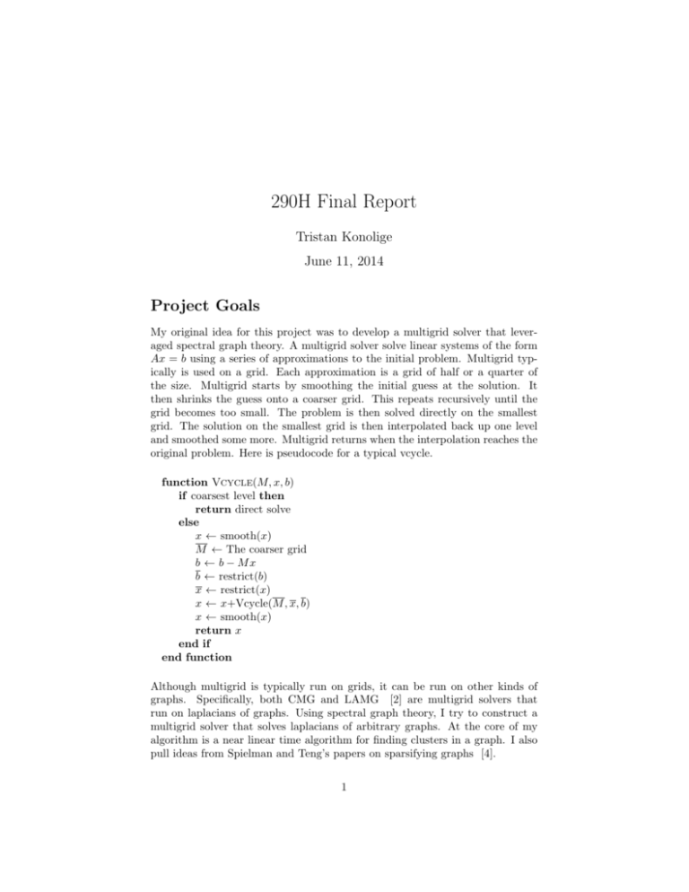
290H Final Report
Tristan Konolige
June 11, 2014
Project Goals
My original idea for this project was to develop a multigrid solver that leveraged spectral graph theory. A multigrid solver solve linear systems of the form
Ax = b using a series of approximations to the initial problem. Multigrid typically is used on a grid. Each approximation is a grid of half or a quarter of
the size. Multigrid starts by smoothing the initial guess at the solution. It
then shrinks the guess onto a coarser grid. This repeats recursively until the
grid becomes too small. The problem is then solved directly on the smallest
grid. The solution on the smallest grid is then interpolated back up one level
and smoothed some more. Multigrid returns when the interpolation reaches the
original problem. Here is pseudocode for a typical vcycle.
function Vcycle(M, x, b)
if coarsest level then
return direct solve
else
x ← smooth(x)
M ← The coarser grid
b ← b − Mx
b ← restrict(b)
x ← restrict(x)
x ← x+Vcycle(M , x, b)
x ← smooth(x)
return x
end if
end function
Although multigrid is typically run on grids, it can be run on other kinds of
graphs. Specifically, both CMG and LAMG [2] are multigrid solvers that
run on laplacians of graphs. Using spectral graph theory, I try to construct a
multigrid solver that solves laplacians of arbitrary graphs. At the core of my
algorithm is a near linear time algorithm for finding clusters in a graph. I also
pull ideas from Spielman and Teng’s papers on sparsifying graphs [4].
1
The Nibble Algorithm
Nibble is a near linear time algorithm for finding low conductance clusters near
a given node in a graph. Nibble’s running time is O(2b(log6 m)/θ4 ). Nibble
works by running an approximate truncated random walk from a starting vertex
[3]. If the walk does not mix rapidly, then Nibble will return a set with low
conductance. Conductance is defined as:
Φ(S) =
|E(S, V − S)|
min(vol(S), vol(V − S))
Where vol is the volume of the set:
X
degree(i)
i∈S
Conductance measures the ratio between the number of edges leaving a set
vs the number of edges in that set. How good of a set Nibble finds is controlled
by the parameter θ. Nibble with find a set with conductance of at most θ or
return an empty set. The size of the set Nibble find is controlled by b. Nibble
will find a set of at most size 2b .
Problems with Nibble
For small values of θ, Nibble can run for too many iterations. Nibble runs
dlog2 (vol(V )/2)e ∗ d
p
2
ln(200(dlog2 (vol(V )/2)e + 2) vol(V )/2e
2
θ
random walk steps before it will return an empty set. If θ is small and there
is no set of conductance θ then θ22 becomes very large. This becomes an issue
later on when I implement the sparsification algorithm presented by Spielman
and Teng [4]. To combat this issue, I fixed the number of iterations to a
constant. Theoretically this makes Nibble less likely to find the correct set,
but in practice it made no difference. The graphs I worked with were not large
enough to require a cut of such low conductance. Furthermore, I only care about
very quick results.
Nibble has a variety of fixed constants. Spielman and Teng [3] provide
constraints on these values and give suitable values. These constants govern
number of iterations, size of truncated values in the random walk, and stopping
conditions. While the provided constants worked fine in practice, I believe that
a better choice of values would improve performance of Nibble.
On graphs with narrow width, the random steps of Nibble can quickly cover
the entire graph. This is not optimal for performance. Furthermore, my implementation of Nibble used a very slow algorithm for computing each random
step. When I scaled up my graph sizes during tests, each random step would
take seconds. This is clearly unacceptable for a ”fast” clustering algorithm.
A quick solution was to truncate the search more aggressively. However, this
sacrificed likelihood of finding a good set of low conductance.
2
Modified Nibble
The version of Nibble I’m using has some significant changes from the original.
function Nibble(G, v, θ, b) v is a vertex
0<θ<1
b is a positive integer
← 1/(c3 (l + 2)tlast 2b )
. Constants are defined in [3]
q ← The vector with a 1 at position v
for t ← 1 to 100 do
q ← [M q]
. A single step of random walks
if there exists a j such that
Φ(Sj (q)) ≤ θ,
vol(Sj ) ≤ (5/6)vol(V ),
2b ≤ vol(Sj ),
q[j] ≥ 1/(c4 (l + 2)2b )
then return Sj
end if
end for
end function
Notice that the loop runs a maximum of 100 times.
Partitioning with Nibble
Nibble can be used to partition a graph. The algorithm for partitioning is
fairly simple. Nibble is repeatedly called with random starting vertices. The
results are unioned with previous Nibbles to form the cut. This procedure is
stopped when the cut reaches the desired size. By taking advantage of Nibble,
the partition algorithm runs in O(m log(1/p) log7 m/θ4 . This algorithm is later
used to sparsity the graph.
Spectral Sparsification
One possible way to perform aggregation is by sparsifying the initial graph. By
removing edges of a graph, we can get an approximating of the original. This
is governed by which defines an partial ordering on graphs. is defined as
follows:
G H ⇐⇒ xT LG x ≤ xT LH x ∀x
If G H then we can use G as an approximating of H. Spielman and Teng [4]
provides an algorithm that takes advantage of this to create sparsified versions
of graphs. This algorithm uses the partitioning algorithm presented above.
Partition is repeated called to approximate a sparse cut in the graph. The
results are then joined together to get a good approximation at the cut. There
3
is a high likelihood that partition find a large cut or overlaps with much of the
sparsest cut [4]. Given a small sparsest cut, it is likely that the complement
is a subgraph of high conductance [4]. Using this fact Spielman and Teng
[4] construct a recursive algorithm to sparsity a graph. If a graph has high
conductance, then it can be approximated by randomly sampling its edges with
probability relative to the minimum degree of the vertices connected by the
edge. They repeatedly call their approximate cut algorithm. If a small cut is
returned, they randomly the complement, otherwise they recursively proceed
on each side of the cut. Using this algorithm, a theoretical running time of
O(m log(1/p) log1 5n) is achieved.
Issues with Sparsification
The sparsification algorithm presented by Spielman and Teng has a few issues
that showed up when I attempted to implement it. - The starting conductance
for Sparsify was too low for all graph I tested. Sparsify uses a starting conductance of 2∗log 1 vol(V ) . Given a 5x5 grid graph with volume 100, starting
29/28
conductance is 3.8×10−3 . There is no set in this graph that has conductance less
than or equal to 3.8×10−3 . For all the graphs I tested, this caused the algorithm
to terminate without sparsifying the graph. By fixing the starting conductance
to a relatively high value, I was able to make Sparsify find nonempty sets in the
graph.
Like Nibble, Sparsify has a number of constants. Unlike Nibble, suitable
constants for these values are not given. These constants govern the stopping
conditions for Sparsify (c3 ) and the conductance value passed to Nibble (c4 ).
I initially tested values of 1 for both of these. Using c3 = 1, Sparsify would
immediately hit its stopping condition without sparsifying any of the graph.
By tweaking c3 ’s value I was able to get Sparsify to not stop immediately on
my test graphs. However, c3 had to be set on a graph by graph basis. This
is not acceptable for a practical algorithm. My stopgap solution was to terminate recursion when the graph achieved a desired size. The other constant,
c4 proved to be useless. c4 governs how much the desired conductance shrinks
when attempting to find an approximate cut in the graph. This shrinkage of
conductance presents its own problem and is discussed in the next issue.
1
At each call to partition, the conductance passed is 1000
of the starting
conductance. As partition is called on a subgraph of the original graph, it would
make more sense to increase conductance rather that decrease it. However, this
reduction in conductance can serve as a stopping condition on the recursion.
Trying to find smaller cuts is more likely to return an empty set, stopping
Sparsify from continuing to partition. This reduction in conductance does not
work in practice. As mentioned earlier, sets with conductance less than or
equal to this reduced value do not exist. This causes Nibble and Partition to
return empty sets before Sparsify has recursed at all. Furthermore, passing low
conductance values to Nibble causes it to run for many iterations. This makes
the algorithm run at a glacial pace. It may be possible to reduce conductance
4
by a reasonable value and get results. In an attempt to get Sparsify to return
a reasonable sparsified graph, I removed the reduction of conductance. This
allowed Sparsify to return results.
The results returned by my modified version of Sparsify were not satisfactory.
All of the time, the sparsified graph returned was not fully connected. This is
most likely not a bug in the original algorithm, but a bug in my implementation
of it. While I spent some time looking for it, I could not find it. I decided that
there was an easier way to use Nibble and Partition in my multigrid scheme.
Nibble for restriction
Multigrid requires a way to approximate a graph with a smaller graph. Spectral graph theory defines a partial ordering on graphs using the . Can I construct a restriction operator that finds a G such that G L? I know that
Spielman and Teng solve this problem by removing edges from the graph. However, when I implemented the Sparsify algorithm it required parameter turning
to even return results. Even once it returned results, these results did not work
in multigrid. When used in my multigrid scheme, interpolation would increase
the residual instead of decreasing it. This is most likely because my Sparsify algorithm does not work correctly. As mentioned above, it always returns graphs
that are not fully connected. Instead I thought I could find a different restriction operator. While Spielman and Teng remove edges to sparsify a graph, I
merge vertices together. This is similar to what happens with restriction on
the model problem. In a one dimensional grid, the size of the grid is halved
with every restriction. The typical 1-D restriction scheme is shown in the figure
above. Notice how three adjacent nodes are merged into one node. I use Nibble
to find sets of vertices to merge. The intuition is that Nibble returns sets of low
conductance. That means vertices in the set are more likely to be closer to each
other than other to other vertices in the graph.
The algorithm I use for restriction is simple. Nibble is called on random
vertices until there are no vertices that are not in a Nibble set. The pseudocode
for that is here:
5
function coarsen(G, θ, b)
S←V
D←∅
while |S| > |V5 | do
v ← a node selected at random from S
N ← Nibble(G, v, θ, b)
Append N to D
S ← S−D
end while
. The set of all vertices
. A set of sets
G0 ← empty graph
for every set si in D do
for every vertex v in s do
for every other set sj in S do
if v ∈ sj thenadd an edge from i to j to G0
end if
end for
end for
end for
return (G0 , D)
end function
Sets returned by Nibble can overlap. This is not an issue. In multigrid on a
grid, restricted sets all overlap. All sets returned by Nibble will be about the
same size. Nibble is guaranteed to return a set around 2b . In my tests, I used
b = 2. This gives set of around 4. Another option is to select b with probability
such that b is in the range [1, 3]. This is the approach that Spielman and Teng
take. In the future, I plan to to try various other values of b.
The coarsen algorithm code only solves the problem of constructing the
coarser graph. However, we still need to restrict x and b to get vectors that fit the
coarser graph. The weighting scheme on a one dimensional grid is [1/4, 1/2, 1/4].
The 1/4 overlaps with the neighbors. I could not find any good theory on restriction in multigrid. One thing I noticed is that the sum of all the ratios add
up to 1. Keeping this in mind, this is what I came up with this for my restriction
operator:
function restrict(S, x)
. S is the set of sets constructed in coarsen
x ← vector of all 0s
for set si in S do
for vertex v in si do
x[i] ← x[i] + x[i]/|si |
end for
end for
return x
end function
6
This restriction scheme works fairly well in practice. For a path graph like
the one dimensional grid, my restriction operator is exactly the same as the
typical restriction operator. In the future I believe I could add the degree of
each node to the restriction operator.
Here is the complete vcycle using Nibble:
function vcycle(G, x, b, θ, p)
if coarsest level then
return direct solve
else
x ← smooth(x)
G ← coarsen(G, θ, p)
b ← b − Gx
b ← restrict(G, b)
x ← restrict(G, x)
x ← x+vcycle(G, x, b, θ, p)
x ← smooth(x)
return x
end if
end function
Performance of this algorithm is still in flux. Currently, interpolating up from
a coarser grid increase error instead of decreasing it. Furthermore, the restricted
b loses orthogonality to the null space. This causes smoothing operations to do
no work.
Future Work
Clearly, there is still a lot of work to be done. My first goal is to make the
restriction operator maintain orthogonality of b. This is most likely the reason
why my multigrid scheme is not working. I need to further experiment with the
restriction operator. I believe that weighting nodes in restriction by their degree
might have a benefit. The slowest part of my multigrid algorithm is Nibble.
The slowness is due to my implementation. Improving my implementation of
Nibble would have a huge difference on the speed of the multigrid algorithm.
An alternative is to implement Nibble-Pagerank by [1]. This algorithm is
functionally equivalent to Nibble but runs in faster time.
Both Nibble and Sparsify have constants that govern how they run. Experimenting with different values for these constants might yield improvements on
accuracy and running time. I would like to throw an optimizer at the constants
and see what values it returns across multiple graphs.
7
References
[1] Reid Andersen, Fan Chung, and Kevin Lang. Local graph partitioning using
pagerank vectors. In Foundations of Computer Science, 2006. FOCS’06.
47th Annual IEEE Symposium on, pages 475–486. IEEE, 2006.
[2] Oren E Livne and Achi Brandt. Lean algebraic multigrid (lamg): Fast graph
laplacian linear solver. SIAM Journal on Scientific Computing, 34(4):B499–
B522, 2012.
[3] Daniel A Spielman and Shang-Hua Teng. A local clustering algorithm for
massive graphs and its application to nearly-linear time graph partitioning.
arXiv preprint arXiv:0809.3232, 2008.
[4] Daniel A Spielman and Shang-Hua Teng. Spectral sparsification of graphs.
SIAM Journal on Computing, 40(4):981–1025, 2011.
8