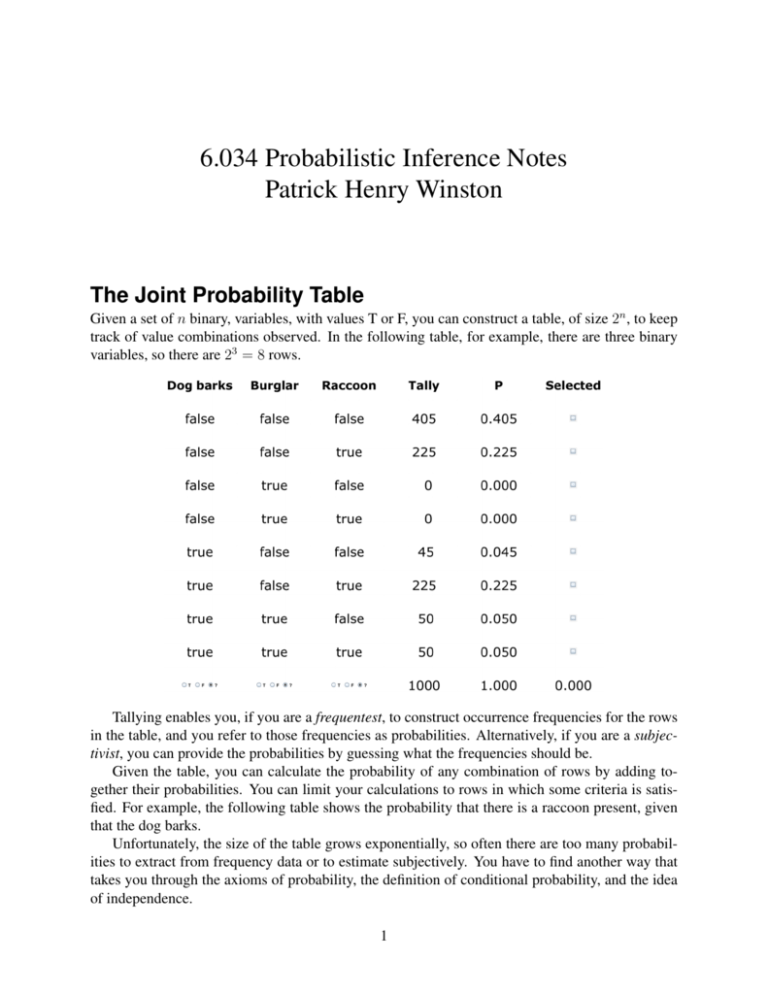
6.034 Probabilistic Inference Notes
Patrick Henry Winston
The Joint Probability Table
Given a set of n binary, variables, with values T or F, you can construct a table, of size 2n , to keep
track of value combinations observed. In the following table, for example, there are three binary
variables, so there are 23 = 8 rows.
Tallying enables you, if you are a frequentest, to construct occurrence frequencies for the rows
in the table, and you refer to those frequencies as probabilities. Alternatively, if you are a subjectivist, you can provide the probabilities by guessing what the frequencies should be.
Given the table, you can calculate the probability of any combination of rows by adding together their probabilities. You can limit your calculations to rows in which some criteria is satisfied. For example, the following table shows the probability that there is a raccoon present, given
that the dog barks.
Unfortunately, the size of the table grows exponentially, so often there are too many probabilities to extract from frequency data or to estimate subjectively. You have to find another way that
takes you through the axioms of probability, the definition of conditional probability, and the idea
of independence.
1
The Axioms of Probability
The axioms of probability make sense intuitively given the capacity to draw Venn diagrams filled
with a colored-pencil crosshatching. The first axiom states that probabilities are always equal to or
greater than zero and less than or equal to one:
0 ≤ P (a) ≤ 1.0
Another axiom captures the idea that certainty means a probability of one; impossible, zero:
P (F ) = 0.0
P (T ) = 1.0
Finally, you have an axiom relating the either (∨) to the both (∧);
P (a ∨ b) = P (a) + P (b) − P (a ∧ b)
Conjunction is generally indicated by a comma, rather than ∧:
P (a, b) = P a ∧ b
Conditional Probability and the Chain Rule
Conditional probability is defined thusly:
P (a|b) ≡
P (a, b)
P (b)
In English, the probability of a given that b is true equals by definition the probability of a and
b divided by the probability of b.
2
Intuitively, this is the probability of a in the restricted universe where b is true. Again, you can
help your intuition to engage by deploying a colored pencil.
Of course you can multiply to get another form of the same definition:
P (a, b) = P (a|b)P (b)
Given the multiplied-out form, note that, by thinking of z as a variable that restricts the universe, you have:
P (a, b, z) = P (a|b, z)P (b, z)
But then, you can work on this expression a little more using the multiplied-out form of the
definition of conditional probability on P (b, z), which yields:
P (a, b, z) = P (a|b, z)P (b|z)P (z)
Once you see this pattern, you can generalize to the chain rule:
P (xn ), ...P (x1 ) = Πi=1
i=n P (xi |xi−1 , ..., x1 ) = P (xn |xn−1 , ..., x1 )P (xn−1 |xn−2 , ..., x1 ) × ... × P (x1 )
The Definition of Independence
The variable a is said, by definition, to be independent of b if:
P (a|b) = P (a)
Thus, independence ensures that the probability of a in the restricted universe where b is true
is the same as the probability of a in the unrestricted universe.
Next, you generalize independence to conditional independence, and define a to be independent
of b given z:
P (a|b, z) ≡ P (a|z)
And then, given the definition, it follows that
P (b|a, z) = P (b|z)
P (a, b, z) = P (a|z)P (b|z)
and
Inference Nets
An inference net is a loop-free diagram that provides a convenient way to assert independence
conditions. They often, but not always, reflect causal pathways:
When you draw such a net, you suggest that the influences on a variable all flow through the
variable’s parents, thus enabling the following to be said: Each variable in an inference net is
independent of all nondescendant variables, given the variable’s parents.
Note that the burglar and raccoon each appear with probabilities that do not depend on anything
else, but the dog barks with differing probabilities depending on whether the burglar or the raccoon
or both or neither are present.
3
The probabilities and conditional probabilities in the diagram are determined using the data to
provide frequencies for all the possibilities, just as when creating the joint probability table.
Using the inference net, there are far fewer numbers to determine with frequency data or to
invent subjectively. Here, there are just 10 instead of 25 = 32 numbers to make up. In general,
if there are n variables, and no variable depends on more than pmax parents, then you are talking
about n2pmax rather than 2n , a huge, exponential difference.
Generating a Joint Probability Table
Is the inference net enough to do calculation? You know that the joint probability table is enough,
so it follows, via the chain rule, that an inference net is enough, because you can generate the rows
in the joint probability table from the corresponding inference net.
To see why, note that, because inference nets have no loops, each inference net must have a
variable without any descendants. Pick such a variable to be first in an ordering of the variables.
Then, delete that variable from the diagram and pick another. There will always be one with no
still-around descendents until you have constructed a complete ordering. No variable in your list
can have any descendents to its right; the descendents, by virtue of how you constructed the list,
are all to the left.
Next, you use the chain rule to write out the probability of any row in the joint probability table
in terms of the variables in your inference net, ordered as you have just laid them out.
For example, you can order the variables in the evolving example by chewing away at the
variables without still-around descendants, producing, say, C, D, B, T, R. Then, using the chain
rule, you produce the following equation:
P (C, D, B, T, R) = P (C|D, B, T, R)P (D|B, T, R)P (B|T, R)P (T |R)P (R)
With this ordering, all the conditional dependencies are on non descendants. Then, knowing
that the variables are independent of all non descendants given their parents, we can strike out a lot
4
of the apparent dependencies, leaving only dependencies on parents:
P (C, D, B, T, R) = P (C|D)P (D|B, R)P (B)P (T |R)P (R)
Thus, it is easy to get the probability of any row in the joint probability table; thus, it is easy to
construct the table; thus, anything you need to infer can be inferred via the inference net.
You need not actually create the full joint probability table, but it is comforting to know that
you can, in principle. You don want to, in practice, because there are ways of performing your
inference calculations that are more efficient, especially if your net has at most one path from any
variable to any other.
Naive Bayes Inference
Now, it is time to revisit the definition of conditional probability and take a walk on a path that will
soon come back to inference nets. By symmetry, note that there are two ways to recast P (a, b):
P (a, b) = P (a|b)P (b)
P (a, b) = P (b|a)P (a)
This leads to the famous Bayes rule:
P (a|b) =
P (b|a)P (a)
P |b)
Now, suppose you are interested in classifying the cause of some observed evidence. You use
Bayes rule to turn the probability of a class, ci , given evidence into the probability of the evidence
given the class, ci :
P (ci |e) =
P (e|ci )P (ci )
P (e)
Then, if the evidence consists of a variety of independent observations, you can write the naive
Bayes classifier, so called because the independence assumption is often unjustified:
P (ci |e1 , ...en ) =
P (e1 |ci ) × ... × P (en |ci ) × P (ci )
P (e)
Of course, if you are trying to pick a class from a set of possibilities, the denominator is the
same for each, so you can just conclude that the most likely class generating the evidence is the
one producing the biggest numerator.
Using the naive Bayes classification idea, you can go after many diagnosis problems, from
medical diagnosis to understanding what is wrong with your car.
5
Model selection
Using the naive Bayes idea, you can also search for the best model given some data. Consider again
the inference net we have been working with. Suppose a friend complains you have it wrong, and
the correct model is the one on the right, not the one on the left:
No problem. You only need use your data to fill in the probabilities, then think of the probabilities of each data element for each classes. Assuming both models are equally likely, all you need
do, for each class, is multiply out the probabilities, in the manner indicated by naive Bayes. The
bigger product indicates the winning class.
Structure search
Next, you develop a program for perturbing inference nets, construct a search program, and look
for the structure that is most probable. You should prepare for some work and frustration, however,
as a simple search is unlikely to work very well. The space is large and full of local maxima and the
potential to models that overfit. You will need random restart and a way to favor fewer connections
over more connections, which you can think of as a special case of Occam’s razor.
6