Towards Unsupervised Whole-Object Segmentation:
Combining Automated Matting with Boundary Detection
Andrew N. Stein∗ Thomas S. Stepleton Martial Hebert
The Robotics Institute, Carnegie Mellon University
Pittsburgh, Pennsylvania 15213, USA
anstein@cmu.edu
Abstract
Input Image
We propose a novel step toward the unsupervised segmentation of whole objects by combining “hints” of partial
scene segmentation offered by multiple soft, binary mattes.
These mattes are implied by a set of hypothesized object
boundary fragments in the scene. Rather than trying to find
or define a single “best” segmentation, we generate multiple segmentations of an image. This reflects contemporary
methods for unsupervised object discovery from groups of
images, and it allows us to define intuitive evaluation metrics for our sets of segmentations based on the accurate and
parsimonious delineation of scene objects. Our proposed
approach builds on recent advances in spectral clustering,
image matting, and boundary detection. It is demonstrated
qualitatively and quantitatively on a dataset of scenes and is
suitable for current work in unsupervised object discovery
without top-down knowledge.
Segmentation "Hints"
High−Probability
Boundary Fragments
Pairwise Affinities
...
...
Object Segmentation
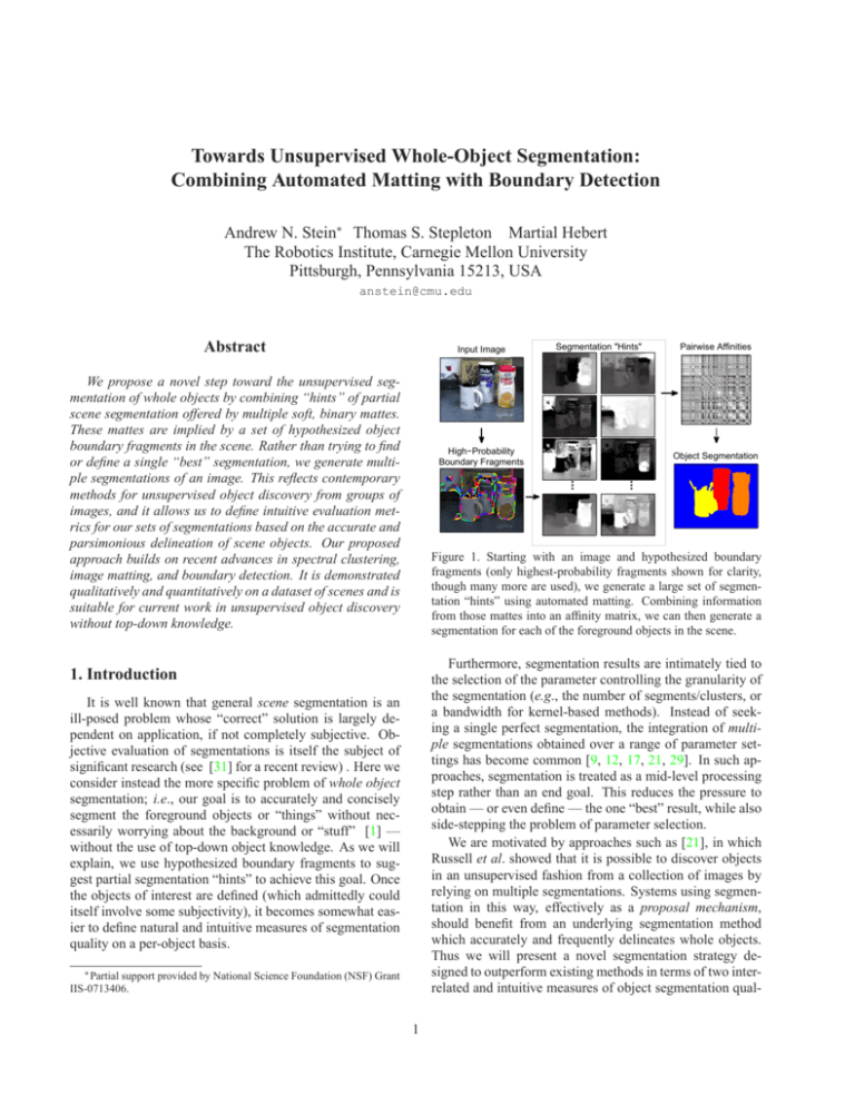
Figure 1. Starting with an image and hypothesized boundary
fragments (only highest-probability fragments shown for clarity,
though many more are used), we generate a large set of segmentation “hints” using automated matting. Combining information
from those mattes into an affinity matrix, we can then generate a
segmentation for each of the foreground objects in the scene.
Furthermore, segmentation results are intimately tied to
the selection of the parameter controlling the granularity of
the segmentation (e.g., the number of segments/clusters, or
a bandwidth for kernel-based methods). Instead of seeking a single perfect segmentation, the integration of multiple segmentations obtained over a range of parameter settings has become common [9, 12, 17, 21, 29]. In such approaches, segmentation is treated as a mid-level processing
step rather than an end goal. This reduces the pressure to
obtain — or even define — the one “best” result, while also
side-stepping the problem of parameter selection.
We are motivated by approaches such as [21], in which
Russell et al. showed that it is possible to discover objects
in an unsupervised fashion from a collection of images by
relying on multiple segmentations. Systems using segmentation in this way, effectively as a proposal mechanism,
should benefit from an underlying segmentation method
which accurately and frequently delineates whole objects.
Thus we will present a novel segmentation strategy designed to outperform existing methods in terms of two interrelated and intuitive measures of object segmentation qual-
1. Introduction
It is well known that general scene segmentation is an
ill-posed problem whose “correct” solution is largely dependent on application, if not completely subjective. Objective evaluation of segmentations is itself the subject of
significant research (see [31] for a recent review) . Here we
consider instead the more specific problem of whole object
segmentation; i.e., our goal is to accurately and concisely
segment the foreground objects or “things” without necessarily worrying about the background or “stuff” [1] —
without the use of top-down object knowledge. As we will
explain, we use hypothesized boundary fragments to suggest partial segmentation “hints” to achieve this goal. Once
the objects of interest are defined (which admittedly could
itself involve some subjectivity), it becomes somewhat easier to define natural and intuitive measures of segmentation
quality on a per-object basis.
∗ Partial support provided by National Science Foundation (NSF) Grant
IIS-0713406.
1
ity. First, we take into account accuracy in terms of pixelwise, per-object agreement between segments. Second, we
also consider conciseness in terms of the number of segments needed to capture an object.
Following the classical Gestalt view as well as Marr’s
theories, we recognize that a key cue in differentiating objects from each other and their background lies in the discovery of their boundaries. Therefore we use hypothesized
fragments of boundaries as input for our segmentations.
Certainly there exists substantial prior work in directly exploiting boundary reasoning for object/ scene segmentation
and figure-ground determination, e.g. [18] and references
therein. Recently, however, Stein et al. [26] have argued
for the importance of detecting physical boundaries due to
object pose and 3D shape, rather than relying on more typical, purely appearance-based edges, which may arise due
to other phenomena such as lighting or surface markings.
They have demonstrated improved boundary detection using cues derived from a combination of appearance and
motion, where the latter helps incorporate local occlusion
information due to parallax from a dynamic scene/ camera.
We employ this method for generating the necessary boundary information for our approach.
Not only do boundaries indicate the spatial extent of objects, however, they also suggest natural regions to use in
modeling those objects’ appearances. The pixels on either
side of a boundary provide evidence which, though only local and imperfect, can offer a “hint” of the correct segmentation by indicating discriminative appearance information.
In practice, we use the output offered by recent αmatting approaches as an approximate “classification”
which realizes these segmentation hints. And though the
individual mattes only suggest binary discrimination (usually “foreground” vs. “background”), we can nevertheless
segment arbitrary numbers of objects in the scene by utilizing the collective evidence offered by a large set of mattes.
Recently, there has been a surge of interest and impressive results in interactive matting [2, 4, 6, 11, 22, 28]. Using
only a sparse set of user-specified constraints, usually in the
form of “scribbles” or a “tri-map”, these methods produce a
soft foreground/ background matte of the entire image. As
initially demonstrated in [3], such methods can potentially
be automated by replacing user-specified “scribbles” with
constraints indicated by local occlusion information.
In the proposed approach, we use each hypothesized
boundary fragment to provide the matting constraints.
Based on the combination of the set of mattes suggested
by all of the fragments, we then derive an affinity measure
which is suitable for use with any subsequent clustering algorithm, e.g. Normalized Cuts (NCuts) [24]. Through this
combination of individually-weaker sources of information
(i.e. fragmented boundaries and impoverished, binary mattes), we relieve the pressure to extract the one “perfect”
matte or the “true” set of extended boundary contours, and
yet we are still able to segment multiple objects in the scene
accurately and concisely. Though beyond the scope of this
work, it is our hope that such improved segmentation strategies will benefit methods which rely on multiple segmentations to generate, for example, object models from unlabeled data.
2. Segmentation “Hints” via Multiple Mattes
As discussed in Section 1, we will use image matting to
produce segmentation “hints” for generating affinities useful in segmentation via clustering. After first providing an
overview of matting, we will explain how we use boundary fragments to imply multiple mattes for estimating these
affinities.
2.1. α-Matting
In a standard matting approach, one assumes that each
observed pixel in an image, I(x, y), is explained by the
convex combination of two unknown colors, F and B. A
soft weight, α, controls this combination:
I(x, y) = α(x, y)F (x, y) + (1 − α(x, y)) B(x, y)
(1)
We will use this model as a proxy for a classifier in our
work. In this formulation, then, pixels with an α-value near
one are likely part of the F “class”, while those with an
α-value near zero are likely part of the B “class”. Values
near 0.5 indicate mixed pixels whose “membership” may
be considered unknown. Typically, F and B correspond
to notions of “foreground” and “background”, but we will
explain in the next section that these semantic assignments
are not necessary for our approach.
Simultaneously solving for F , B, and α in (1) is of
course not feasible. In general, a user specifies a small set
of pixels, often referred to as “scribbles” or a “tri-map”,
which are then constrained to belong to one class or the
other. These hard constraints are then combined with assumptions about α (e.g., smoothness) to find a solution at
the unspecified pixels [2, 4, 6, 11, 22, 28]. We have adopted
the approach proposed by Levin et al. [11], which offers excellent results via a closed-form solution for α based on reasonable assumptions about the local distributions of color in
natural images.
Note that methods also exist for constrained “hard” segmentations, e.g. [5] — potentially with some soft matting
at the boundaries enforced in post-processing [20] — but as
we will see, using fully-soft α-mattes allows us to exploit
the uncertainty of mixed pixels (i.e. those with α values near
0.5) rather than arbitrarily (and erroneously) assigning them
to one class or the other. In fact, we follow the conventional
wisdom of avoiding early commitment throughout our approach. Hard thresholds or grouping decisions are avoided
in favor of maintaining soft weights until the final segmentation procedure. In addition to retaining the maximum
amount of information for the entire process, this methodology also avoids the many extra parameters required for
typical ad hoc decisions or thresholds.
2.2. Multiple Mattes → Affinities
In an automated matting approach, the goal is to provide
a good set of constraints without requiring human intervention. Since object boundaries separate two different objects
by definition, they are natural indicators of potential constraint locations: F on one side and B on the other. In [3],
T-junctions were used to suggest sparse constraints in a similar manner. The benefit of matting techniques here is their
ability to propagate throughout the image the appearance
information offered by such local, sparse constraints. The
middle of Figure 1 depicts a sampling of mattes generated
from the differing constraints (or “scribbles”) implied by
various boundary fragments.
A remaining problem is that the approach described
thus far only offers a binary (albeit soft) decision about a
pixel’s membership: it must belong to either F or B, which
are usually understood to represent foreground and background. How then can we deal with multi-layered scenes?
We recognize that the actual class membership of a particular pixel, as indicated by its α value in a single matte,
is rather meaningless in isolation. What we wish to capture, however, is that locations with similar α values across
many different mattes (whether both zero or one) are more
likely to belong to the same object, while locations with
consistently different values are more likely to be part of
different objects. While existing methods, such as Intervening Contours [7, 8, 10], may attempt to perform this type of
reasoning over short- and medium-ranges within the image
using standard edge maps, our use of mattes simultaneously
factors in the boundaries themselves as well as the global
appearance discrimination they imply. Furthermore, matte
values near 0.5 carry a notion of uncertainty about the relationship between locations.
Using each of the NF potential boundary fragments in
the scene to generate an image-wide matte yields an NF length vector, vi , of α-values at each pixel i. If we scale
the α-values to be between +1 and −1 (instead of 0 and
1), such that zero now represents “don’t know”, then the
agreement, or affinity, between two pixels i and j can be
written in terms of the normalized correlation between their
two scaled matting vectors:
Aij =
viT W vj
,
|vi ||vj |
(2)
where W is a diagonal matrix of weights corresponding to
the confidence of each fragment actually being an object
boundary. Thus mattes derived from fragments less likely
to be object boundaries will not significantly affect the final
affinity. Note that this combines all hypothesized fragments
in a soft manner, avoiding the need to choose some ideal
subset, e.g., via thresholding. Figure 2 provides an example schematic describing the overall process of employing
boundary fragments to suggest mattes, which in turn generate an affinity matrix.
The value of Aij will be maximized when the matting
vectors for a pair of pixels usually put them in the same
class. When a pair’s vectors usually put the two pixels in
opposite classes, the affinity will be minimized. The normalization effectively handles discounting the “don’t know”
(near-zero) entries which arise from mattes that do not provide strong evidence for one or both pixels of the pair.
We have now defined a novel matting-based affinity measure which can be used with any off-the-shelf clustering
technique. In addition to incorporating boundary knowledge and global appearance reasoning, a unique and noteworthy aspect of our affinities is that they are defined based
on feature vectors in a space whose dimension is a function
of the image content — i.e. the number of detected fragments, NF — rather than an arbitrarily pre-defined feature
space of fixed dimension.
3. Detecting Boundary Fragments
In the previous section, we constructed mattes based on
hypothesized boundary fragments. We will now explain the
source of these hypotheses. While one could use a purely
appearance-based edge detector, such as P b [13], as a proxy
for suggesting locations of object boundaries in a scene,
this approach could also return many edges corresponding
to non-boundaries, such as surface markings, yielding extra
erroneous and misleading mattes. While it would be naı̈ve
to expect or require perfect boundary hypotheses from any
method, we still wish to maximize the fraction that do indeed correspond to true object boundaries.
Recently, Stein et al. demonstrated improved detection
of object/ occlusion boundaries by incorporating local, instantaneous motion estimates when short video clips are
available [26, 27]. Their method first over-segments a scene
into a few hundred “super-pixels” [19] using a watershedbased approach. All super-pixel boundaries are used as potential object boundary fragments (where each fragment begins and ends at the intersection of three or more superpixels). Using learned classifiers and inference on a graphical model, they estimate the probability that each fragment
is an object boundary based on appearance and motion cues
extracted along the fragment and from within each of the
neighboring super-pixels. The resulting boundary probabilities provide the weights for W in (2). An example input
image and its boundary fragments (shown in differing colors), can be found on the left side of Figure 1. For clarity,
only the high-probability fragments are displayed, though
we emphasize that all are used.
For each fragment, we can now generate an image-wide
matte according to [11] as described in Section 2. The
super-pixels on either side of a fragment naturally designate
spatial support for the required labeling constraints. Since
super-pixels generally capture fairly homogeneous regions,
however, we have found it better to expand the constraint
set for a fragment by using a triplet of super-pixels formed
by also incorporating the super-pixels of the two neighboring fragments most likely to be boundaries. This process is
i
B
vi
F
Aij
F
F
Compare
B
j
B
vj
Boundary Fragments → Matting Constraints
Segmentation "Hints" → Feature Vectors
Pairwise Comparisons → Affinity Matrix
Figure 2. Each potential boundary fragment found in the original image (three shown here) implies a set of constraints (F and B) used to
generate a matte. Vectors of matting results at each location in the image (vi and vj ) can be compared in a pairwise fashion to generate an
affinity matrix, A, suitable for clustering/ segmentation.
illustrated in Figure 3. Note also that our approach avoids
any need to choose the “right” boundary fragments (e.g. by
thresholding), nor does it attempt to extract extended contours using morphological techniques or an ad hoc chaining
procedure, both of which are quite brittle in practice. Instead we consider only the individual short fragments, with
an average length of 18 pixels in our experiments.
We employ the technique proposed in [26, 27] in order
to improve our performance by offering better boundary detection and, in turn, better mattes. As mentioned above,
that approach utilizes instantaneous motion estimates near
boundaries. We are not, however, incorporating motion estimates (e.g. optical/ normal flow) directly into our segmentation affinities [23, 32], nor is our approach fundamentally
tied to the use of motion.1
Pr = 0.4
Pr = 0.3
F
F
F
Pr = 0.8
F
B
Pr = 0.1
B
Pr = 0.7
B
B
Pr = 0.2
Figure 3. The F and B constraint sets for a given fragment are
initialized to its two neighboring super-pixels (left). To improve
the mattes, these constraint sets are expanded to also include the
super-pixels of the fragment’s immediate neighbors with the highest probability of also being object boundaries (right).
4. Image Segmentation by NCuts
Given our pairwise affinity matrix A, which defines a
fully-connected, weighted graph over the elements in our
image, we can use spectral clustering according to the Normalized Cut Criterion to produce an image segmentation
with K segments [24].2 To obtain a set of multiple segmentations, we can simply vary this parameter K.
1 Separate experiments using P b alone to supply the weights in W
yielded reasonable but slightly worse results than those presented in Section 6. This suggests that both the better boundaries from [26, 27] and the
matting-based affinities presented here are useful.
2 Certainly other techniques exist, but NCuts is a one popular one that
also offers mature, publicly-available segmentation methods, facilitating
the comparisons in Section 6. Our work is not exclusively tied to NCuts.
Using the boundary-detection approach described above,
we not only obtain a better set of hypothesized boundary
fragments and probabilities of those fragments corresponding to physical object boundaries (i.e. for use in W from
(2)), but we can also use the computed super-pixels as our
basic image elements instead of relying on individual pixels. In addition to offering improved, data-driven spatial
support, this drastically reduces the computational burden
of constructing Aij , making it possible to compute all pairwise affinities between super-pixels instead of having to
sample pixelwise affinities very sparsely.
The benefit here is more than reduced computation, however, particularly when using the popular NCuts technique.
Other authors have noted that non-intuitive segmentations
typical of NCuts stem from an inability to fully populate
the affinity matrix and/or the topology of a simple, fourconnected, pixel-based graph [30]. By computing affinities
between all pairs of super-pixels, we alleviate somewhat
both of these problems while also improving speed.
We will not review here all the details of spectral clustering via NCuts, given a matrix of affinities; see [14] for
specifics of the method we follow. We compare the segmentations obtained using NCuts on our matting-based affinities to two popular approaches from the literature, each of
which also uses NCuts and offers an implementation online.
First is the recent multiscale approach of Cour et al. [7],
in which affinities are based on Intervening Contours [10].
Second, we compare to the Berkeley Segmentation Engine
(BSE) [8, 13], which relies on a combined set of patchbased and gradient-based cues (including Intervening Contours). Note that different methods exist for the final step of
discretizing the eigenvectors of the graph Laplacian. While
the BSE uses k-means (as do we, see [14]), the multiscale
NCuts method attempts to find an optimal rotation of the
normalized eigenspace [34]. Furthermore, both methods
compute a sparsely-sampled, pixelwise affinity matrix.
5. Evaluating Object Segmentations
In this section, we will present an intuitive approach for
determining whether one set of segmentations is “better”
than another generated using a different method. For the
eventual goal of object segmentation and discovery, we propose that the best set of segmentations will contain at least
one result for each object in the scene in which that object can be extracted accurately and with as few segments
as possible. Ideally, each object would be represented by a
single segment which is perfectly consistent with the shape
of that object’s ground truth segmentation. We leave the
problem of identifying the object(s) from sets of multiple
segmentations to future work and methods such as [21].
Thus, we define two measures to capture these concepts:
consistency and efficiency. For consistency, we adopt a
common metric for comparing segmentations, which conveniently lies on the interval [0, 1] and captures the degree
to which two sets of pixels, R and G, agree based on their
intersection and union:
|R ∩ G|
.
(3)
c(R, G) =
|R ∪ G|
Here, R = {A, B, C, . . . } ⊆ S is a subset of segments
from a given (over-)segmentation S, and G is the ground
truth object segmentation.
At one extreme, if our segmentation were to suggest a
single segment for each pixel in the image, we could always
reconstruct the object perfectly by selecting those segments
(or in this case, pixels) which corresponded exactly to the
ground-truth object’s segmentation. But this nearly-perfect
consistency would come at the cost of an unacceptably high
number of constituent segments, as indicated in the rightmost example in Figure 4. At the opposite extreme, our
segmentation could offer a single segment which covers the
entire object, as shown in the leftmost example. In this case,
we would achieve the desired minimum of one segment to
capture the whole object, but with very poor consistency.
Number of
Segments Required
1
3
250+
6
Inreasing Segmentation Consistency
Figure 4. The tradeoff between segmentation consistency (or accuracy) and efficiency (or the number of segments required to
achieve that consistency). As desired consistency increases, so too
does the number of segments required to achieve that consistency.
Thus we see that there exists a fundamental tradeoff between consistency and the number of segments needed to
cover the object, or efficiency.3 Therefore, when evaluat3 It may be helpful to think of these measures and their tradeoff as being
roughly analogous to the common notions of precision and recall, e.g., in
object recognition.
ing the quality of a scene’s (over-)segmentation S, we must
take into account both measures. We define the efficiency
as the size of the minimal subset of segments, R, required
to achieve a specified desired consistency, cd , according to
the ground truth object segmentation, G:
ecd (S, G) = min |R|, such that c(R, G) ≥ cd .
(4)
Note that with this definition, a lower value of e(S, G) implies a more efficient (or parsimonious) segmentation.
We can now specify cd and compute the corresponding
ecd , which is equivalent to asking, “what is the minimum
number of segments required to achieve the desired consistency for each object in this scene?” By asking this question
for a variety of consistency levels, we can evaluate the quality of a particular method and compare it to other methods’
performance at equivalent operating points.
Note that we can avoid a combinatorial search over all
subsets R possibly required to achieve a particular cd by
considering only those segments which overlap the ground
truth object and by imposing a practical limit on the number
of segments we are willing to consider (selected in order of
their individual consistency measures) [27].
Referring once again to Figure 4, the middle two examples indicate that we can achieve a reasonable level of
consistency with only three segments, and if we raise the
desired consistency a bit higher (perhaps in order to capture the top of the mug), it will require us to use a different
segmentation from our set which covers the mug with six
segments. In general, the best method would be capable of
providing at least one segmentation which yields a desired
high level of consistency with the minimum degree of oversegmentation of any particular object.
6. Experiments
For each of a set of test scenes, we have labeled the
ground truth segmentation for foreground objects of interest, which we roughly defined as those objects for which
the majority of their boundaries are visible. Since we employ [26]’s method for boundary information, we also use
their online dataset of 30 scenes. From those scenes, we
have labeled ground truth segmentations for 50 foreground
objects on which we will evaluate our approach.
We generate a set of segmentations for each scene by
varying K between 2 and 20 while using either our mattingbased approach, multiscale NCuts [7], or the BSE approach [8, 13]. Recall that the two latter methods compute affinities in a pixelwise fashion. To verify that any
improvement offered by our approach is not solely due to
our use of super-pixels, we also implemented a baseline
approach which computes affinities from pairwise comparisons of L*a*b* color distributions within each super-pixel,
using the χ2 -distance.
For our proposed approach, we use each of the individual boundary fragments from [26] to suggest constraints for
mattes as described in Section 2.2. In practice, we ignore
Segments Required to Achieve Specified Consistency
Color Distribution Affinity
Multiscale NCuts
Berkeley Segmentation Engine (BSE)
Proposed Matting−Based Affinity
# Segments Required
Not Possible
10
9
8
7
6
5
4
3
2
1
0
0.5
0.55
0.6
0.65
0.7
0.75
0.8
0.85
0.9
0.95
Desired Object Segmentation Consistency
Ground Truth Object
Super−Pixels
High−Probability
Boundary Fragments
Color
Distribution
Multiscale NCuts
BSE
Our Proposed
Matting Affinity
cd ≥ 0.70
Input Image
c=0.71, ec=5.00
c=0.79, ec=3.00
c=0.71, ec=2.00
Not Possible
Not Possible
c=0.71, ec=1.00
cd ≥ 0.80
those fragments with an extremely low probability (< 0.01)
of being boundaries, since the resulting mattes in those
cases would have almost no effect on computed affinities
anyway. From an initial set of 350-1000, this yields approximately 90-350 fragments (and mattes) per image for
computing pairwise, super-pixel affinities according to (2).
We first selected a set of ten desired consistency levels,
from 0.5 to 0.95. Then for each labeled object in a scene and
for each segmentation method, we pose the question, “what
is the minimum number of segments required to achieve
each desired consistency in segmenting this object?” We
can then graph and compare the methods’ best-case efficiencies as a function of the desired consistencies.
A typical graph is provided at the top of Figure 5, in
which bars of different colors correspond to different segmentation methods. Each group of bars corresponds to a
certain consistency level, and the height of the bars indicates the minimum efficiency (i.e. number of segments required) to achieve that consistency. Thus, lower bars are
better. Bars extend to the top of the graph when a method
could not achieve a desired consistency with any number of
segments. Thus we see that our approach is able to achieve
similar consistency with fewer segments — until cd reaches
0.85, at which point all methods fail on this image. Not surprisingly, the relatively simplistic appearance model of the
color-only baseline tends to over-segment objects the most.
We can also examine the actual segmentations produced
by each method at corresponding desired consistency levels, as shown at the bottom of Figure 5. For the input image
and selected ground truth object shown we provide for each
method the segmentations which use the minimum number
of segments and achieved at least the desired consistency
indicated to the left of the row. Also shown are the superpixels used for our method and the color-distribution approach, along with a high-probability subset of the boundary fragments used in the proposed approach. (We display
only a subset of the fragments actually used simply for clarity.) Below each segmentation are the actual consistencies
and efficiencies (i.e. number of segments) obtained. Note
how our method achieves comparable consistencies with
fewer segments — even when other methods may not be
able to achieve that consistency at all. More results are provided in Figures 6-7 and in the supplemental material.
Not surprisingly, when the desired consistency is low,
any method is usually capable of capturing an object with
few segments. But as the desired consistency increases, it
becomes more difficult, or even impossible, to find a small
number of segments to recover that object so accurately.
Finally, as the desired consistency becomes too high, all
methods begin to fail. We find, however, that for many objects our matting-based approach tends to maintain better
efficiency (i.e. decreased over-segmentation) into a higherconsistency regime than the other methods.
To capture this more quantitatively over all objects, we
can compute the difference between the number of seg-
c=0.81, ec=9.00
c=0.81, ec=3.00
Figure 5. Top: A typical graph of segmentation efficiency vs. consistency for a set of desired consistency levels. Our method is able
to achieve similar object segmentation consistency with fewer segments. Bottom: The corresponding input data (first row) and the
resulting segmentations at two consistency levels (2nd , 3rd rows),
as indicated by cd = {0.70, 0.80} to the left of each row. For
clarity, only high-probability boundary fragments used by our approach are shown, using a different color for each fragment. For
visualization, the individual segments corresponding to the object,
i.e. those used to compute the c and e values displayed below
each segmentation, have been colored with a red-yellow colormap,
while background segments are colored blue-green.
ments our method requires at each consistency level and the
number required by the other methods. We would like to
see that our method often requires significantly fewer segments to achieve the same consistency. Certainly, there are
some “easier” objects for which the choice of segmentation
method may not matter, so we would also expect to find that
our method regularly performs only as well as other methods. But we also must ensure that we do better much more
often than worse. Furthermore, we expect the potential benefit of our approach to be most obvious within a reasonable
range of desired consistency: all methods will tend to perform equally well at low consistencies, and all methods will
tend to fail equally often at very high consistencies.
Figure 8 offers evidence that our approach does indeed
outperform the other methods as desired. As expected, we
perform just as well (or poorly) as other methods for many
of the objects, particularly at very low or very high desired
consistency. But we require several fewer segments per object in a significant number of cases. Furthermore, our approach rarely hurts; we do not often require more segments
than the other methods.
Segments Required to Achieve Specified Consistency
Not Possible
10
9
8
7
6
5
4
3
2
1
0
Color Distribution Affinity
Multiscale NCuts
Berkeley Segmentation Engine (BSE)
Proposed Matting−Based Affinity
9
8
7
# Segments Required
# Segments Required
Not Possible
6
5
4
3
2
1
0
0.5
0.55
0.6
0.65
0.7
0.75
0.8
0.85
0.9
Segments Required to Achieve Specified Consistency
Color Distribution Affinity
Multiscale NCuts
BSE
Proposed Matting−Based
0.5
0.55
0.6
0.65
0.7
0.75
0.8
Desired Object Segmentation Consistency
Ground Truth Object
Super−Pixels
Color
Distribution
Multiscale NCuts
BSE
Our Proposed
Matting Affinity
c=0.74, ec=5.00
c=0.72, ec=6.00
c=0.71, ec=2.00
c=0.72, ec=1.00
c=0.83, ec=7.00
Not Possible
c=0.82, ec=4.00
c=0.83, ec=3.00
0.9
0.95
Input Image
Ground Truth Object
Super−Pixels
High−Probability
Boundary Fragments
Color
Distribution
Multiscale NCuts
BSE
Our Proposed
Matting Affinity
c=0.69, ec=2.00
c=0.65, ec=2.00
c=0.72, ec=3.00
c=0.84, ec=1.00
c=0.76, ec=10.00
Not Possible
c=0.81, ec=4.00
c=0.84, ec=1.00
cd ≥ 0.80
cd ≥ 0.80
cd ≥ 0.70
cd ≥ 0.65
Input Image
High−Probability
Boundary Fragments
0.85
Desired Object Segmentation Consistency
0.95
Figure 6. Another example showing our method’s ability to
achieve comparable consistency with fewer segments.
Figure 7. Another example like those in Figures 5-6. Note only
one of the three objects in the scene is shown here.
Discussion & Conclusion
yielded very good results, but it was fickle: when it failed,
it often failed completely. Future research in this direction
is certainly warranted, however.
Debate continues over whether high-level reasoning, e.g.
object recognition, should precede figure-ground perception [15], or if purely bottom-up, local reasoning can account for this process [16, 25]. Our work takes the more
bottom-up perspective, since knowledge of specific objects
is not required (unlike [18]), but our use of matting incorporates more powerful, semi-global reasoning as compared to purely-local methods. Our experiments indicate
that by maintaining “soft” reasoning throughout, and by
combining multiple, individually-imperfect sources of information in the form of fragmented boundary hypotheses
and oft-uncertain mattes, our novel method for addressing
object segmentation yields promising results for use in subsequent work on unsupervised object discovery or scene understanding. While here we have evaluated our affinities in
isolation, as compared to existing methods, it is certainly
possible that combining multiple types of affinities would
offer further improvement.
Using boundaries and mattes as described simultaneously implies the grouping and separation of super-pixels
on the same or opposite sides of a given boundary, respectively. We performed preliminary experiments with
the technique described in [33] to incorporate separately
such “attraction” and “repulsion” evidence via spectral clustering, rather than simply treating the two as equivalent
sources of information with opposite signs. This often
References
[1] E. H. Adelson and J. R. Bergen. The plenoptic function and
the elements of early vision, chapter 1. The MIT Press, 1991.
[2] N. E. Apostoloff and A. W. Fitzgibbon. Bayesian video matting using learnt image priors. In CVPR, 2004.
[3] N. E. Apostoloff and A. W. Fitzgibbon. Automatic video
segmentation using spatiotemporal T-junctions. In BMVC,
2006.
[4] X. Bai and G. Sapiro. A geodesic framework for fast interactive image and video segmentation and matting. In ICCV,
2007.
[5] Y. Boykov and M. P. Jolly. Interactive graph cuts for optimal
boundary and region segmentation of objects in N-D images.
In ICCV, 2001.
[6] Y. Chuang, B. Curless, D. Salesin, and R. Szeliski. A
bayesian approach to digital matting. In CVPR, 2001.
[7] T. Cour, F. Bénézit, and J. Shi. Spectral segmentation with
multiscale graph decomposition. In CVPR, 2005.
[8] C. Fowlkes, D. Martin, and J. Malik. Learning affinity functions for image segmentation: Combining patch-based and
gradient-based approaches. In CVPR, 2003.
[9] D. Hoiem, A. A. Efros, and M. Hebert. Recovering surface
layout from an image. IJCV, 75(1), October 2007.
[10] T. Leung and J. Malik. Contour continuity in region based
image segmentation. In ECCV, June 1998.
Improvement
Performance of "Matting: Simple NCuts" vs. Other Approaches
Color Distribtions
As Compared to:
Multiscale NCuts
BSE
Fraction of Objects
1
Desired Consistency of 0.60
0.8
Degradation Summary:
For 12% of the objects, we require
average of 1.6 MORE segments
0.6
0.4
Improvement Summary:
For 27% of the objects, we require
average of 2.5 FEWER segments
0.2
0
<= −5
−4
−3
−2
−1
0
+1
+2
+3
+4
>= +5
Fraction of Objects
1
Desired Consistency of 0.70
0.8
Degradation Summary:
For 11% of the objects, we require
average of 1.1 MORE segments
0.6
0.4
Improvement Summary:
For 42% of the objects, we require
average of 3.4 FEWER segments
0.2
0
<= −5
−4
−3
−2
−1
0
+1
+2
+3
+4
>= +5
Fraction of Objects
1
Desired Consistency of 0.80
0.8
Degradation Summary:
For 7% of the objects, we require
average of 1.7 MORE segments
0.6
0.4
Improvement Summary:
For 58% of the objects, we require
average of 4.0 FEWER segments
0.2
0
<= −5
−4
−3
−2
−1
0
+1
+2
+3
+4
>= +5
cd
0.50
0.55
0.60
0.65
0.70
0.75
0.80
0.85
0.90
0.95
∆e
2.0
2.3
2.5
2.7
3.4
3.8
4.0
3.6
4.2
4.7
% Obj.
21%
26%
27%
34%
42%
47%
58%
39%
30%
11%
Degradation
−∆e
1.3
1.4
1.6
1.2
1.1
1.9
1.7
2.1
3.5
3.4
% Obj.
3%
6%
12%
10%
11%
11%
7%
12%
9%
5%
For each desired consistency level cd , we indicate the percentage of objects for which
we offer improvement over other methods
and how many fewer segments we require
on average (∆e) — higher values are better for both. Similarly, for cases where we
do worse, we indicate how many more segments we require (−∆e) and how often —
lower values are better here.
Relative Number of Segments Required by Other Method
Figure 8. Overall Performance. At left are histograms of the relative number of segments required by our approach as compared to the
other methods. The height of the bars corresponds to the fraction of the total number of objects for which we achieve the specified relative
efficiency on the x-axis. Thus, bars at zero, in the center of the graph, correspond to cases when we perform just as well as the other
approaches. Bars to the right (left) correspond to cases where we perform better (resp., worse), using fewer (resp., more) segments than
the competition. The table and the insets on the graphs provide summary statistics at the specified consistency levels.
[11] A. Levin, D. Lischinski, and Y. Weiss. A closed form solution to natural image matting. In CVPR, 2006.
[12] T. Malisiewicz and A. A. Efros. Improving spatial support
for objects via multiple segmentations. In BMVC, 2007.
[13] D. R. Martin, C. C. Fowlkes, and J. Malik. Learning to detect
natural image boundaries using local brightness, color, and
texture cues. POCV, 26(5):530–549, May 2004.
[14] A. Y. Ng, M. I. Jordan, and Y. Weiss. On spectral clustering:
Analysis and an algorithm. In NIPS, 2001.
[15] M. A. Peterson and B. S. Gibson. Must figure-ground organization precede object recognition? An assumption in peril.
Psychological Science, 5(5):253–259, September 1994.
[16] F. T. Qiu and R. von der Heydt. Figure and ground in the
visual cortex: V2 combines stereoscopic cues with gestalt
rules. Neurons, 47:155–166, July 2005.
[17] A. Rabinovich, A. Vedaldi, and S. Belongie. Does image
segmentation improve object categorization? Cs2007-0908,
University of California San Diego, 2007.
[18] X. Ren, C. C. Fowlkes, and J. Malik. Figure/ground assignment in natural images. In ECCV, 2006.
[19] X. Ren and J. Malik. Learning a classification model for
segmentation. In ICCV, volume 1, pages 10–17, 2003.
[20] C. Rother, V. Kolmogorov, and A. Blake. “grabCut”: Interactive foreground extraction using iterated graph cuts. SIGGRAPH, 23(3):309–314, 2004.
[21] B. C. Russell, A. A. Efros, J. Sivic, W. T. Freeman, and
A. Zisserman. Using multiple segmentations to discover objects and their extent in image collections. In CVPR, 2006.
[22] M. Ruzon and C. Tomasi. Alpha estimation in natural images. In CVPR, 2000.
[23] J. Shi and J. Malik. Motion segmentation and tracking using
normalized cuts. In ICCV, pages 1154–1160, 1998.
[24] J. Shi and J. Malik. Normalized cuts and image segmentation. POCV, 22(8):888–905, August 2000.
[25] L. Spillmann and W. H. Ehrenstein. Gestalt factors in the
visual neurosciences. In L. M. Chalupa and J. S. Werner,
editors, The Visual Neurosciences, pages 1573–1589. MIT
Press, Cambridge, MA, November 2003.
[26] A. Stein, D. Hoiem, and M. Hebert. Learning to find object
boundaries using motion cues. In ICCV, 2007.
[27] A. N. Stein. Occlusion Boundaries: Low-Level Processing to
High-Level Reasoning. Doctoral dissertation, The Robotics
Institute, Carnegie Mellon University, February 2008.
[28] J. Sun, J. Jia, C.-K. Tang, and H.-Y. Shum. Poisson matting.
SIGGRAPH, 23(3):315–321, 2004.
[29] J. Tang and P. Lewis. Using multiple segmentations for image auto-annotation. In ACM International Conference on
Image and Video Retrieval, 2007.
[30] D. A. Tolliver and G. L. Miller. Graph partitioning by spectral rounding: Applications in image segmentation and clustering. In CVPR, 2006.
[31] R. Unnikrishnan, C. Pantofaru, and M. Hebert. Toward objective evaluation of image segmentation algorithms. POCV,
29(6):929–944, June 2007.
[32] J. Xiao and M. Shah. Accurate motion layer segmentation
and matting. In CVPR, 2005.
[33] S. Yu and J. Shi. Segmentation with pairwise attraction and
repulsion. In ICCV, July 2001.
[34] S. X. Yu and J. Shi. Multiclass spectral clustering. In ICCV,
2003.