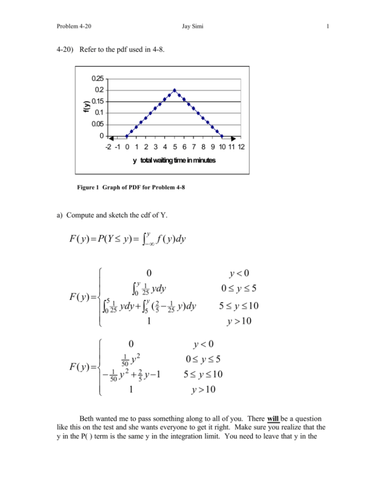
Problem 4-20
Jay Simi
1
4-20) Refer to the pdf used in 4-8.
0.25
f(y)
0.2
0.15
0.1
0.05
0
-2 -1 0 1 2 3 4 5 6 7 8 9 10 11 12
y total waiting time in minutes
Figure 1 Graph of PDF for Problem 4-8
a) Compute and sketch the cdf of Y.
F ( y) = P(Y ≤ y) =
y
∫− ∞ f ( y) dy
0

y 1

ydy
∫

0 25
F ( y) =  5
y 2
1
1
∫0 25 ydy + ∫5 ( 5 − 25 y) dy

1
0


1 y2

F ( y) =  1 502 2
− 50 y + 5 y −1

1
y<0
0≤ y≤5
5 ≤ y ≤ 10
y > 10
y<0
0≤ y ≤5
5 ≤ y ≤ 10
y > 10
Beth wanted me to pass something along to all of you. There will be a question
like this on the test and she wants everyone to get it right. Make sure you realize that the
y in the P( ) term is the same y in the integration limit. You need to leave that y in the
Problem 4-20
Jay Simi
2
integration because the CDF is a function and not a number. When you are looking for a
probability over a given interval, then you replace the y with a value and solve it.
1.2
1
F(y)
0.8
0.6
0.4
0.2
0
0
2
4
6
8
10
12
y total waiting time in minutes
Figure 2 Graph of CDF for the PDF from Problem 4-8
b) Obtain an expression for the (100p)th percentile.
Percentiles represent the area of the graph of f(y) that lies to the left of a given value.
For example, η(.75), the 75th percentile, is such that the area under the graph of f(y)
to the left of η(.75) is .75.
η ( p)
P (Y ≤ η ( p)) = p = F (η ( p)) = ∫−∞ f ( y) dy
For p < .5
F (η ( p )) =
y2
50
=p
η ( p) = 5 2 p
2
For p > .5
y
F (η ( p )) = − 50
+ 25 y − 1 = p
η ( p) =
2
5
1 )(1 − p )
± ( 25 ) 2 − 4 ( 50
2
50
η ( p) = 10 ± 2(1 − p)
Problem 4-20
Jay Simi
3
c) Compute E(Y) and V(Y).
∞
E ( y) = ∫−∞ y ∗ f ( y) dy
=
5 y2
0 25
(Page 150)
10
∫
dy + ∫5 ( 25 y − 251 y 2 ) dy
y3 5
= 75 | 0 + ( 15
= 5 minutes
y2 −
1
75
y 3 ) |10
5
V (Y ) = E (Y 2 ) − [ E (Y )]2
E (Y 2 ) = y 2 ∗ f ( y )dy
5 y3
=
0 25
∫
10 2
(
5 5
dy + ∫
(Page 150)
y −
2
y4
) dy
25
2
= 29.167 minutes
V(Y) = 29.167 minutes 2 - (5 minutes) 2
V(Y) = 4.167 minutes 2
0.25
The expected value of
5 makes sense
because the graph is
symmetric about 5.
f(y)
0.2
0.15
0.1
0.05
0
-2 -1 0 1 2 3 4 5 6 7 8 9 10 11 12
y total waiting time in minutes
Figure 3 Graph of PDF from Problem 4-8
How do these values compare with those for a single bus when the time is uniformly
distributed on [0,5]?
Whereas Y had previously been used to represent the waiting time for two buses,
now I have to define a new rv.
Let X = time to wait for one bus
X j uniform(0,5)
Problem 4-20
Jay Simi
 1
f ( x; A, B ) =  B − A
 0
0≤x≤5
otherwise
Uniform distribution is defined as:
1
f ( x; 0, 5) =  5
0
4
A≤ x≤ B
otherwise
5
E ( X ) = ∫0 15 xdx
x 2 |5
= 10
0
= 2.5 minutes
V ( X ) = E ( X 2 ) − [ E ( X )] 2
5
E ( X 2 ) = ∫0 15 X 2 dx
x 3 |5
= 15
0
= 25
min 2
3
V ( X ) = 253 − 2.52
V ( X ) = 2.08 min 2
The values for the uniform distribution were half of those seen for the previous
distribution. This makes sense because Y is the sum of two uniformly distributed
random variables. Y is the waiting time for two buses and X is the waiting time form
one bus.
Y = X1 + X 2
So….
E (Y ) = E ( X 1 ) + E ( X 2 )
V (Y ) = E ( X 1 ) + E ( X 2 )