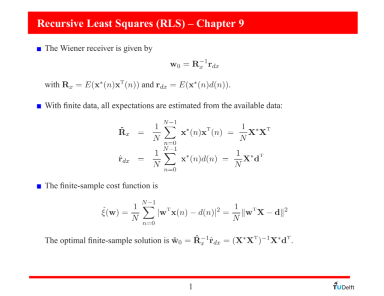
Recursive Least Squares (RLS) – Chapter 9
The Wiener receiver is given by
w0 = R−1
x rdx
with Rx = E(x∗ (n)xT (n)) and rdx = E(x∗ (n)d(n)).
With finite data, all expectations are estimated from the available data:
R̂x =
r̂dx =
N −1
1 X ∗
1 ∗ T
T
x (n)x (n) =
X X
N
N
n=0
N
−1
1 X ∗
1 ∗ T
x (n)d(n) =
X d
N
N
n=0
The finite-sample cost function is
N
−1
X
1
1
T
T
ˆ
|w x(n) − d(n)|2 = kw X − dk2
ξ(w)
=
N
N
n=0
∗ T −1 ∗ T
The optimal finite-sample solution is ŵ0 = R̂−1
x r̂dx = (X X ) X d .
1
Matrix inversion lemma
H
H
H
( A − B C−1 B )−1 = A−1 + A−1 B (C − BA−1 B )−1 BA−1 .
P ROOF


A B
H
B C


 = 
I B C−1

0

H

0

BA−1 I

0

−C−1 B I

= 




A B
H
B C
A B
H
B C
−1

−1


= 

= 

= 
I
I
I
I −A−1 B
0
I
H

H
A − B C−1 B
C
A
C − BA−1 BH
H
( A − B C−1 B )−1

0

C−1 B I

A−1 BH

I

I


0

I
0
0

C−1


A−1

(C − BA−1 BH )−1
A−1 + A−1 BH (C − BA−1 BH )−1 BA−1 ∗
∗
2
∗



H
I −B C−1

0
I

I
0
−BA−1 I


The RLS algorithm
Xn := [x(0), · · · , x(n)] ,
Suppose at time n we know
dn := [d(0), · · · , d(n)]
The solution to min k wT Xn − dn k2 is
ŵ(n) = (X∗n Xn )−1 X∗n dn
T
T
=:
Φ−1
n θn
where
T
Φn := X∗n Xn =
n
X
T
T
x∗ (i)x (i) ,
θ n := X∗n dn =
i=0
n
X
x∗ (i)d(i)
i=0
Update of Φ−1
n :
Φ−1
n+1
∗
T
= (Φn + x (n + 1)x (n + 1))
−1
=
Φ−1
n
T
∗
−1
Φ−1
n x (n + 1)x (n + 1)Φn
−
∗
1 + xT (n + 1)Φ−1
n x (n + 1)
Recursive Least Squares (RLS) algorithm:
Pn x∗ (n + 1)xT (n + 1)Pn
−
1 + xT (n + 1)Pn x∗ (n + 1)
Pn+1
:= Pn
θ n+1
:= θ n + x∗ (n + 1)d(n + 1)
ŵ(n+1) := Pn+1 θ n+1
Initialization: θ 0 = 0 and P0 = δ −1 I, where δ is a very small positive constant.
3
The RLS algorithm
Finite horizon
For adaptive purposes, we want an effective window of data.
1. Sliding window: Φn and θ n based on only the last L samples:
T
T
Φn+1 = Φn + x∗ (n + 1)x (n + 1) − x∗ (n − L)x (n − L)
θ n+1 = θ n + x∗ (n + 1)d(n + 1) − x∗ (n − L)d(n − L)
Doubles complexity, and we have to keep L previous data samples in memory.
2. Exponential window: scale down Φn and θ n by a factor λ ≈ 1:
T
Φn+1 = λΦn + x∗ (n + 1)x (n + 1)
θ n+1 = λθ n + x∗ (n + 1)d(n + 1)
Corresponds to
Xn+1 = [x(n + 1)
λ1/2 x(n)
λx(n − 1) λ3/2 x(n − 2) · · · ]
dk+1 = [d(n + 1)
λ1/2 d(n)
λd(n − 1)
4
λ3/2 d(n − 2) · · · ]
The RLS algorithm
Exponentially weighted RLS algorithm:
−
Pn x∗ (n + 1)xT (n + 1)Pn
1 + λ−1 xT (n + 1)Pn x∗ (n + 1)
Pn+1
:=
θ n+1
:= λθ n + x∗ (n + 1)d(n + 1)
λ−1 Pn
λ−2
ŵ(n+1) := Pn+1 θ n+1
convergence of output error cost function
0.6
RLS
LMS
SGD
0.5
J
0.4
0.3
µ=0.088
0.2
λ=0.7
0.1
λ=1
0
0
50
100
time [samples]
5
150