Using Your TI-NSpire Calculator: Normal Distributions
Dr. Laura Schultz
Statistics I
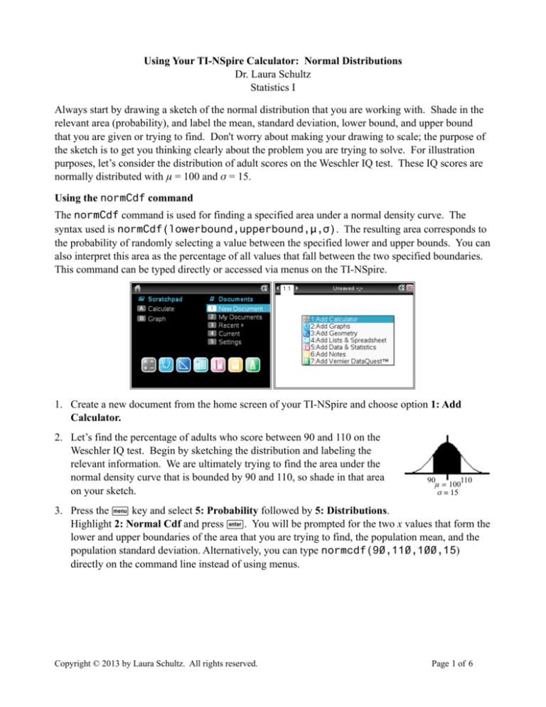
Always start by drawing a sketch of the normal distribution that you are working with. Shade in the
relevant area (probability), and label the mean, standard deviation, lower bound, and upper bound
that you are given or trying to find. Don't worry about making your drawing to scale; the purpose of
the sketch is to get you thinking clearly about the problem you are trying to solve. For illustration
purposes, let’s consider the distribution of adult scores on the Weschler IQ test. These IQ scores are
normally distributed with μ = 100 and σ = 15.
Using the normCdf command
The normCdf command is used for finding a specified area under a normal density curve. The
syntax used is normCdf(lowerbound,upperbound,μ,σ). The resulting area corresponds to
the probability of randomly selecting a value between the specified lower and upper bounds. You can
also interpret this area as the percentage of all values that fall between the two specified boundaries.
This command can be typed directly or accessed via menus on the TI-NSpire.
1. Create a new document from the home screen of your TI-NSpire and choose option 1: Add
Calculator.
2. Let’s find the percentage of adults who score between 90 and 110 on the
Weschler IQ test. Begin by sketching the distribution and labeling the
relevant information. We are ultimately trying to find the area under the
normal density curve that is bounded by 90 and 110, so shade in that area
on your sketch.
90
110
μ = 100
σ = 15
3. Press the b key and select 5: Probability followed by 5: Distributions.
Highlight 2: Normal Cdf and press ·. You will be prompted for the two x values that form the
lower and upper boundaries of the area that you are trying to find, the population mean, and the
population standard deviation. Alternatively, you can type normcdf(90,110,100,15)
directly on the command line instead of using menus.
Copyright © 2013 by Laura Schultz. All rights reserved.
Page 1 of 6
4. Your calculator will return the area under the normal curve bounded by 90 and 110. Thus, we
find that 49.5% of adults score between 90 and 110 on the Weschler IQ test. Remember to round
percentages to three significant figures.
5. What is the probability that a randomly selected adult scores less than 120 on the Weschler IQ
test? Problems like this are a bit trickier because your calculator requires both a lower bound and
an upper bound. What is the lower bound in this case? (You may have noticed that your
calculator uses -∞ as the default lower bound when you use menus to access the normCdf
command, which is helpful for problems like this one.)
6. Start by drawing a sketch. This time, try typing in the command normcdf(-∞,120,100,15)
directly into the calculator rather than using the menus. You can type the
infinity symbol by pressing /k to access a menu of special symbols.
(Be sure to use the v key to specify a negative sign rather than the
subtraction key. ) We find that the probability of randomly selecting an
120
-∞
adult whose IQ is below 120 is 0.909. In symbols, P(x < 120) = 0.909.
μ = 100
σ = 15
Remember to round probability values to 3 significant figures.
7. It is a bit tedious to graph a normal distribution on a TI-Nspire, but it can be done.
Let’s try plotting the adult Weschler IQ distribution and shading in the area for the previous
example. Press ~ and then select 4: Insert followed by 6: Lists & Spreadsheets. Name list
A iq and list B density. Then, press the ~ key again and select 4: Insert followed by 7: Data
& Statistics. Click at the bottom the graph window that appears, and identify the x-axis variable
as iq. Identify the y-axis variable as density.
Copyright © 2013 by Laura Schultz. All rights reserved.
Page 2 of 6
8. Press the b key and select 4: Analyze followed by 4: Plot Function. Type in normPdf(x,
100,15)and press ·. You will need to change the window settings so that the graph is
actually readable. To do this, press b and select 5: Window/Zoom followed by 1: Window
Settings. Experiment until you find the settings that result in the best graph. As a rule of thumb,
pick Xmin and Xmax values that are a bit more that three standard deviations below and above
the mean, respectively. You can get an idea of what to use for YMax by looking at the initial
graph; Ymin should always be 0.
9. We can now shade in the area corresponding to P(x < 120) or any other desired probability. Press
the b key and select 4: Analyze followed by 5: Shade Under Function. Use the touch pad to
select your desired lower limit and click a. Then, move to your desired upper limit and click on
a again. You’ll notice that you can only click on the approximate limits; hence, the numerical
value that is returned along with the shaded graph is only an approximation of the actual area you
were trying to find. In this case, 0.91 is a pretty good approximation of P(x < 120). However,
you should not rely on using a graph to find areas under the normal curve; the results obtained
using the normCdf command are much more accurate. Click anywhere on the screen to hide the
function.
Copyright © 2013 by Laura Schultz. All rights reserved.
Page 3 of 6
10. What percentage of adults score at least 90 on the Weschler IQ test?
Because your calculator requires both a lower bound and an upper bound,
you will need to use ∞ for your upper bound. Hence, the syntax for
problems of this sort is normCdf(lowerbound,∞,μ,σ).
11. Start by drawing a sketch. Go back to the calculator screen
(1.1) and enter the command normcdf(90,∞,
100,15)either directly or by navigating through the relevant
menus on your TI-NSpire.
90
μ = 100
σ = 15
∞
12. We find that 74.8% of adults score at least 90 on the Weschler
IQ test. Remember to round to 3 significant figures.
Using the invNorm command
Use the invNorm command when you are given a probability or percentage and asked to find an x
value. This command is often used to find values corresponding to percentiles or quartiles. Your
calculator requires that you enter the cumulative area to the left of the desired value; drawing a sketch
is very useful for making sure you enter the correct area. Sometimes you will need to work with an
area other than the one specified by the problem.
1. Let’s start by finding the IQ score corresponding to the 95th percentile (P95). Begin by drawing a
sketch and labeling it.
2. Press b and select 5: Probability followed by 5: Distributions. We’ll
be using 3: Inverse Normal. You will be prompted to enter the total area
to the left of the desired x value, µ, and σ. Note that instead of using the
menus, you can type in this command directly using the syntax
invNorm(area to left,μ,σ).
Copyright © 2013 by Laura Schultz. All rights reserved.
Area to left =
0.95
P95
μ = 100
σ = 15
Page 4 of 6
3. Your calculator will return the desired x value. For this example, we find that the Weschler IQ
score corresponding to the 95th percentile is 124.7. Round your answer to one more decimal
place than what was provided for μ.
4. Let’s try a trickier example. This time, find the IQ score separating the top
15% of all Weschler IQ scores from the rest. Start by drawing a sketch.
Given that the total area under the normal density curve is always 1, the
area to the left of the IQ score that we are seeking can be found by
subtracting the given area from 1. In this case, 1 - 0.15 = 0.85. Don’t
forget to convert percentages to their equivalent decimal values.
Area to left =
0.85
x
μ = 100
σ = 15
5. The area to the left of the IQ score we are seeking is 0.85, so
type invNorm(0.85,100,15) and then press ·. We
find that an IQ score of 115.5 separates the top 15% of all
adult Weschler IQ scores from the rest.
Applying the Central Limit Theorem
Working with sample means
• The Central Limit Theorem applies whenever you are working with a distribution of sample means
( x ), and the sample comes from a normally distributed population, and/or the sample size is at
least 30 (n ≥ 30).
• Recall that the mean for a distribution of sample means is µ x = µ , and the standard deviation for a
σ
distribution of sample means is σ x =
.
n
• Thus, the modified calculator commands to use when you are applying the Central Limit Theorem
to work with a distribution of sample means ( x ) are as follows:
normalcdf(lowerbound,upperbound,μ,
normalcdf(-∞,upperbound,μ,
normalcdf(lowerbound,∞,μ,
invNorm(area to left,μ,
Copyright © 2013 by Laura Schultz. All rights reserved.
σ
)
n
σ
)
n
σ
)
n
σ
)
n
Page 5 of 6
Working with sample proportions
• The mean for a distribution of sample proportions is µ p̂ = p , and the standard deviation for a
distribution of sample proportions is σ p̂ =
pq
.
n
• Whenever np ≥ 10 and nq ≥ 10, the sampling distribution of a sample proportion can be
approximated by a normal distribution. (Note that q = 1 - p.)
• The modified calculator commands to use when you are working with a distribution of sample
proportions ( p̂ ) that can be approximated by a normal distribution are as follows:
normalcdf(lowerbound,upperbound,p,
normalcdf(0,upperbound,p,
pq
)
n
normalcdf(lowerbound,1,p,
pq
)
n
invNorm(area to left,p,
Copyright © 2013 by Laura Schultz. All rights reserved.
pq
)
n
pq
)
n
Page 6 of 6
