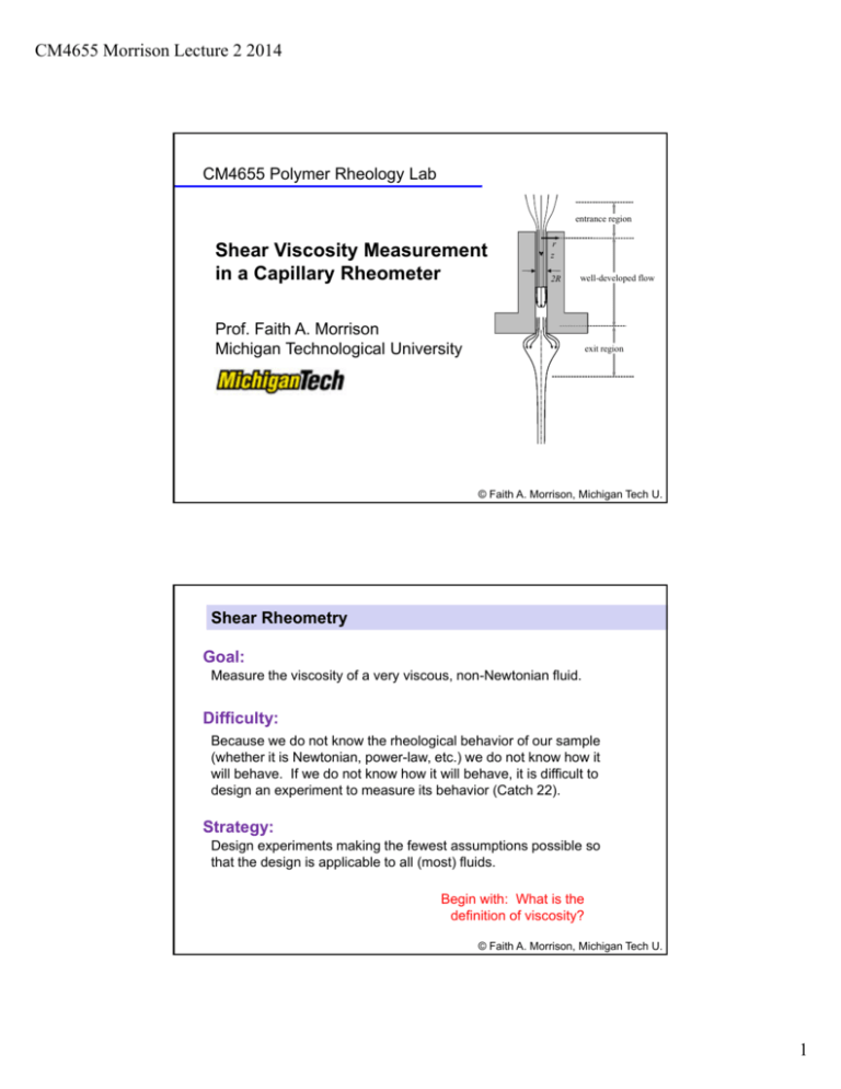
CM4655 Morrison Lecture 2 2014
CM4655 Polymer Rheology Lab
entrance region
Shear Viscosity Measurement
in a Capillary Rheometer
r
z
2R
well-developed flow
Prof. Faith A. Morrison
Michigan Technological University
exit region
1
© Faith A. Morrison, Michigan Tech U.
Shear Rheometry
Goal:
Measure the viscosity of a very viscous, non-Newtonian fluid.
Difficulty:
Because we do not know the rheological behavior of our sample
(whether it is Newtonian, power-law, etc.) we do not know how it
will behave. If we do not know how it will behave, it is difficult to
design an experiment to measure its behavior (Catch 22).
Strategy:
Design experiments making the fewest assumptions possible so
that the design is applicable to all (most) fluids.
Begin with: What is the
definition of viscosity?
2
© Faith A. Morrison, Michigan Tech U.
1
CM4655 Morrison Lecture 2 2014
By definition, viscosity is measured in pure, homogeneous shear flow
force=F
velocity field
shear rate:
v1 ( H )  V  0 H
0 
0  constant
v1 ( x2 )
H
x2
 0 x2 


v  0 
 0 

123
x1
x1 (t  t )
x1 (t )
v1
x2
V
x2
x1

path lines
 21 F / A

0 V / H
3
© Faith A. Morrison, Michigan Tech U.
By definition, viscosity is measured in pure, homogeneous shear flow
Means,
the shear rate
force=F
is the same at every
v1 ( H )  V  0 H
position
in space
velocity field
shear rate:
0  constant
v1 ( x2 )
H
x2
x1
x1 (t )
0 
x1 (t  t )
V
v1
x2
 0 x2 


v  0 
 0 

123
x2
x1
path lines

 21 F / A

0 V / H
4
© Faith A. Morrison, Michigan Tech U.
2
CM4655 Morrison Lecture 2 2014
By definition, viscosity is measured in pure, homogeneous shear flow
Means,
the shear rate
force=F
is the same at every
v1 ( H )  V  0 H
position
in space
velocity field
shear rate:
0 
0  constant
has
v1 ( xThis
x2
2)
the
advantage of
subjecting every
x1 fluid
particle to the same
deformation
x (t  t )
H
x1 (t )
v1
x2
 0 x2 


v  0 
 0 

123
1
V
x2
x1

path lines
 21 F / A

0 V / H
5
© Faith A. Morrison, Michigan Tech U.
By definition, viscosity is measured in pure, homogeneous shear flow
Means,
the shear rate
force=F
is the same at every
v1 ( H )  V  0 H
position
in space
velocity field
shear rate:
0  constant
H
the
advantage of
subjecting every
x1 fluid
particle to the same
deformation
x (t  t )
has
v1 ( xThis
x2
2)
x1 (t )
1
x2
v1
x2
 0 x2 


v  0 
 0 
V

123
(just in case it matters
to the measurement
of viscosity)
x1
path lines
0 

 21 F / A

0 V / H
6
© Faith A. Morrison, Michigan Tech U.
3
CM4655 Morrison Lecture 2 2014
By definition, viscosity is measured in pure, homogeneous shear flow
Means,
the shear rate
force=F
is the same at every
v1 ( H )  V  0 H
position
in space
velocity field
shear rate:
0 
0  constant
has
v1 ( xThis
x2
2)
the
advantage of
subjecting every
x1 fluid
particle to the same
deformation
x (t  t )
H
x1 (t )
1
x2
v1
x2
 0 x2 


v  0 
 0 
V

123
(just in case it matters
to the measurement
of viscosity)
x1
(which it does, for
non-Newtonian fluids)
path lines
7
© Faith A. Morrison, Michigan Tech U.
By definition, viscosity is measured in pure, homogeneous shear flow
force=F
velocity field
shear rate:
v1 ( H )  V  0 H
0 
0  constant
v1 ( x2 )
H
x2
x1
x1 (t )
x1 (t  t )
V
v1
x2
 0 x2 


v  0 
 0 

123
x2
x1
path lines

 21 F / A

0 V / H
8
© Faith A. Morrison, Michigan Tech U.
4
CM4655 Morrison Lecture 2 2014
Drawbacks
•Parallel plate flow is difficult to produce (maintaining constant
gap for example)
•Stress measurements are affected by edge effects and spacers
used to maintain gap
•Signal can be low amplitude (signal-to-noise ratio)
•Sample loading is inconvenient and complex
Even though producing the parallel plate
geometry is tricky, it has been done: J. M.
Dealy and S. S. Soong J. Rheol. 28, 355
(1984); doi:10.1122/1.549756
A Parallel Plate Melt Rheometer
Incorporating a Shear Stress Transducer
Can we use an alternate,
easier geometry?
(Sliding Plate Rheometer)
9
© Faith A. Morrison, Michigan Tech U.
Sliding Plate Rheometer
Image from: www.rheology.org
Image from:
www.mcgill.ca/photos/2006/february/
John Dealy
McGill University
Hee Eon Park, works on a high-pressure sliding
plate rheometer, the only instrument of its kind
in the world.
Even though producing the parallel plate
geometry is tricky, it has been done: J. M.
Dealy and S. S. Soong J. Rheol. 28, 355
(1984); doi:10.1122/1.549756
A Parallel Plate Melt Rheometer
Incorporating a Shear Stress Transducer
(Sliding Plate Rheometer)
10
© Faith A. Morrison, Michigan Tech U.
5
CM4655 Morrison Lecture 2 2014
Shear is fundamentally a sliding flow
We can infer a viscosity from any sliding flow if we can relate the data
back to homogeneous shear flow
x2
Cartesian
geometry
(parallel plates)
x1
Cylindrical
geometry
r
z
R
r1
Telescoping
sliding flow
r2
r3
(capillary flow)
11
© Faith A. Morrison, Michigan Tech U.
Strategy:
Use capillary flow experiments (pressure drop versus
flow rate) to infer viscosity
Implications:
•The flow is not the simple shear flow assumed when viscosity
was defined;
•We need to analyze the flow with as few assumptions as
possible;
•We need to design the apparatus to conform to the assumptions
we make;
•When our assumptions are only approximately satisfied, we
must correct the data where possible.
12
© Faith A. Morrison, Michigan Tech U.
6
CM4655 Morrison Lecture 2 2014
Capillary Rheometer
•Shear viscosity is the most widely measured rheological property
•For high shear rates, the capillary rheometer is the most effective
instrument for measuring shear viscosity.
•The capillary rheometer does not produce pure, homogeneous shear
flow, however.
•Various corrections are necessary in order to turn pressure-drop/flow-rate
data from a capillary rheometer into viscosity.
   ( ) 
 21

Three corrections:
1.
Entrance/exit pressure loss
2.
Slip at the wall
3.
Non-parabolic velocity profile
13
© Faith A. Morrison, Michigan Tech U.
Capillary Rheometer
piston
The basics
F
entrance region
A
barrel
2Rb
polymer melt
reservoir
r
z
2R
well-developed flow
B
exit region
Q
14
© Faith A. Morrison, Michigan Tech U.
7
CM4655 Morrison Lecture 2 2014
Goettfert
Rheo-Tester 1000
15
© Faith A. Morrison, Michigan Tech U.
Classic Newtonian flow problem:
Pressure-driven flow of a fluid in a
tube
•steady state
•well developed
•long tube (no z-dependence)
•no-slip at the wall
For all fluids:
Stress at the wall:
R 
Definition of viscosity:
cross-section A:
r
 
4Q
 R3

 R

P0
z
PR
2L
For Newtonian fluids only:
Shear rate at the wall:
r
z
A
L
vz(r)
fluid
R
PL
16
© Faith A. Morrison, Michigan Tech U.
8
CM4655 Morrison Lecture 2 2014
Newtonian Fluid:
Hagen-Poiseuille law
R 4 P
Q
8L
 4Q  1  PR 
 3 

 R    2 L 
 PR 
 4Q 

   3 
 2L 
 R 
PR
2L

This is only true for
Newtonian fluids.
4Q
R 3
17
© Faith A. Morrison, Michigan Tech U.
Corrections to Capillary flow
• entrance and exit effects - Bagley correction
(correct the pressure drop)
•slip at the wall - Mooney analysis (correct the flow
rate)
(NOTE: we do not do this
correction in CM4655)
•Non-parabolic velocity profile - WeissenbergRabinowitsch correction (correct the shear rate at the
wall; non-Newtonian effects)
18
© Faith A. Morrison, Michigan Tech U.
9
CM4655 Morrison Lecture 2 2014
Entrance and exit effects - Bagley correction
The pressure gradient is not
accurately represented by
the raw p/L
entrance region
r
z
2R
well-developed flow
P(z)
 p 


 L raw
exit region
 p 
 L 

corrected
z=L
z=0
z
19
© Faith A. Morrison, Michigan Tech U.
Entrance and exit effects - Bagley correction
L
PR
R 
 P   2 R   0
2L
R
no
intercept
r
z
Constant at fixeda
Run for different
length capillaries
Straight line through origin with
slope of 2R:
P
2 R
L
R
entrance region
2R
well-developed flow
exit region
This is the
result when
the end
effects are
negligible.
20
© Faith A. Morrison, Michigan Tech U.
10
CM4655 Morrison Lecture 2 2014
Entrance and exit effects - Bagley correction
Procedure:
•For a standard set of apparent shear rates
4Q/R3, measure P in capillaries of different
L/R (usually different lengths)
P   2 R 
L
R
•Plot results and infer corrected shear stress
from slope
P
2 R
L
R
21
© Faith A. Morrison, Michigan Tech U.
Bagley Plot
1200
effects
apparent
a  R  shear
rate
4Q
3
250
Pressure drop (psi)
Pend  f (Q)  f (a )
a ( s 1 )
1000
120
90
800
60
40
600
400
200
Pend
effects   250 s 1
a
0
-10
0
10
20
30
40
L/R
-1
e(250, s )
Figure 10.8, p. 394 Bagley, PE
22
© Faith A. Morrison, Michigan Tech U.
11
CM4655 Morrison Lecture 2 2014
1200
y = 32.705x + 163.53
R2 = 0.9987
Steady State Pressure,
1000
y = 22.98x + 107.72
R2 = 0.9997
800
y = 20.172x + 85.311
R2 = 0.9998
600
y = 16.371x + 66.018
R2 = 0.9998
400
y = 13.502x + 36.81
R2 = 1
200
The intercepts are equal to the
entrance pressure losses.
0
0
10
20
30
40
L/R
23
Figure 10.8, p. 394 Bagley, PE
© Faith A. Morrison, Michigan Tech U.
Figure 10.8, p. 394 Bagley, PE
1200
y = 32.705x + 163.53
R2 = 0.9987
Steady State Pressure,
1000
y = 22.98x + 107.72
R2 = 0.9997
800
y = 20.172x + 85.311
R2 = 0.9998
600
y = 16.371x + 66.018
R2 = 0.9998
400
y = 13.502x + 36.81
R2 = 1
200
0
0
10
20
30
L/R
 rz 
pR
2L
L
 p  2 rz  
R
The slopes are equal to
twice
40 the shear stress for
the various apparent
shear rates
24
© Faith A. Morrison, Michigan Tech U.
12
CM4655 Morrison Lecture 2 2014
The data so far:
Δ
gammdotA deltPent
(1/s)
psi
250
163.53
120
107.72
90
85.311
60
66.018
40
36.81
slope
psi
32.705
22.98
20.172
16.371
13.502
sh stress
psi
16.3525
11.49
10.086
8.1855
6.751
sh stress
Pa
1.1275E+05
7.9220E+04
6.9540E+04
5.6437E+04
4.6546E+04
Now, correct shear rate
for slip at the wall
25
Figure 10.8, p. 394 Bagley, PE
© Faith A. Morrison, Michigan Tech U.
Slip at the wall - Mooney analysis
Slip at the wall reduces the shear
rate near the wall.
v1 ( x2 )
v1 ( x2 )
no slip
x2
 
x1
dv1
dx 2
dv1
dx 2
slip
v1, slip
x2
 
x1
dv1
, smaller
dx 2
dv1
dx 2
26
© Faith A. Morrison, Michigan Tech U.
13
CM4655 Morrison Lecture 2 2014
Slip at the wall - Mooney analysis
Slip at the wall reduces the shear
rate near the wall.
a 
4Q 4v z ,av

R 3
R
without slip
4
vz ,av  vz ,slip 
R
4v z , slip
4v
 z ,av 
R
R
1
 
 4v z , slip    a , slip corrected
R
a ,slip corrected 
4v z ,av
R
4v z ,av
R

4Qmeasured
R 3
slope
with slip
Need
capillaries of
various radii
intercept
27
© Faith A. Morrison, Michigan Tech U.
Slip at the wall - Mooney analysis
800
pR , MPa
2L
4Q
R
600
0.35
0.3
4v z , slip
3
0.25
0.2
-1
(s )
0.14
400
0.1
0.05
0.01
200
0
0
Figure 10.10, p. 396
Ramamurthy, LLDPE
1
2
3
1/R (1/mm)
4
Now, correct shear rate for
non-parabolic velocity profile.
28
© Faith A. Morrison, Michigan Tech U.
14
CM4655 Morrison Lecture 2 2014
For an unknown, non-Newtonian fluid, we need to take
special steps to determine the wall shear rate
The wall shear rate is generally greater for a nonNewtonian fluid than for a Newtonian fluid.
vz(r)
R ,non  Newtonian
Newtonian
velocity profile
non-Newtonian
velocity profile
R, Newtonian
r
29
© Faith A. Morrison, Michigan Tech U.
Weissenberg-Rabinowitsch correction
R ( R ) 
4Q
R 3
1 
d ln a 

  3 
4
d
ln

R

 
10
a 
slope is a
function of R
4Q
R
Sometimes the WR
correction varies from
point-to-point;
sometimes it is a
constant that applies to
all data points.
3
1
slope 
d ln a
d log  R
0.1
0.1
1
PR
R 
2L
10
Procedure: fit a line to
data, differentiate it;
evaluate derivative
function at points of
interest.
30
© Faith A. Morrison, Michigan Tech U.
15
CM4655 Morrison Lecture 2 2014
Weissenberg-Rabinowitsch correction
ln(apparent shear rate, 1/s)
7
For these data,
the derivative is a
constant.
y = 2.0677x - 18.537
R2 = 0.9998
6
5
This slope is
usually >1
d ln a
 2.0677
d ln  R
4
3
10
10.4
Figure 10.8, p. 394 Bagley, PE
10.8
11.2
11.6
12
ln(shear stress, Pa)
31
© Faith A. Morrison, Michigan Tech U.
The data corrected for entrance/exit and nonparabolic velocity profile:

R
R
Δ
deltPent
Δ
sh stress
gammdotA deltPent
ln(sh st)
ln(gda)
WR
gam-dotR viscosity
(1/s)
psi
Pa
Pa
correction
1/s
Pa s
250
163.53 1.1275E+06 1.1275E+05 11.63289389 5.521460918
2.0677 316.73125 3.5597E+02
120
107.72 7.4270E+05 7.9220E+04 11.2799902 4.787491743
2.0677
152.031 5.2108E+02
90
85.311 5.8820E+05 6.9540E+04 11.14966143 4.49980967
2.0677 114.02325 6.0988E+02
60
66.018 4.5518E+05 5.6437E+04 10.9408774 4.094344562
2.0677
76.0155 7.4244E+02
40
36.81 2.5380E+05 4.6546E+04 10.74820375 3.688879454
2.0677
50.677 9.1849E+02
Now, plot viscosity versus
wall-shear-rate
Figure 10.8, p. 394 Bagley, PE
32
© Faith A. Morrison, Michigan Tech U.
16
CM4655 Morrison Lecture 2 2014
Viscosity of polyethylene from Bagley’s data
1.0E+04
R
R
Viscosity, Pa s

1.0E+03
1.0E+02
10
Figure 10.8, p. 394 Bagley, PE
R
100
Shear rate, 1/s
1000
33
© Faith A. Morrison, Michigan Tech U.
Viscosity from Capillary Experiments, Summary:
1. Take data of pressure-drop
versus flow rate for capillaries of
various lengths; perform Bagley
correction (entrance pressure)
3. Perform the WeissenbergRabinowitsch correction (wall
shear rate)
4. Plot true viscosity versus true
wall shear rate
P(Q)
final data:
   R / R
1.0E+04

 R
R
Viscosity, Pa s
2. If slip is an issue, take data for
capillaries of different radii;
perform Mooney correction
(slip)
raw data:
1.0E+03
1.0E+02
10
5. Fit to a power-law to obtain
model parameters if desired.
R
100
Shear rate, 1/s
1000
34
© Faith A. Morrison, Michigan Tech U.
17
CM4655 Morrison Lecture 2 2014
Capillary Rheometer Measurement Procedure
•Choose range of apparent shear rates and capillary sizes to
allow for desired corrections.
•Conduct experiments: load reservoir; push polymer through
capillary with piston
•Measure pressure at top of capillary at the base of the barrel
(correct for entrance and exit losses); obtain wall shear stress.
•Measure piston speed (convert to flow rate, correct for slip);
obtain apparent shear rate.
•Plot apparent shear rate versus wall shear stress; obtain WR
correction
•Correct apparent shear rate for non-parabolic velocity profile
(non-Newtonian)
•Calculate true non-Newtonian viscosity from stress/shear rate.
35
© Faith A. Morrison, Michigan Tech U.
Schedule your lab time with our TA
Week 4
Week 5
• First, one hour to play with the software
• Second, 3 hours to take data
• Third, 3 hours to take remaining data
• Fourth (optional) more data
36
© Faith A. Morrison, Michigan Tech U.
18