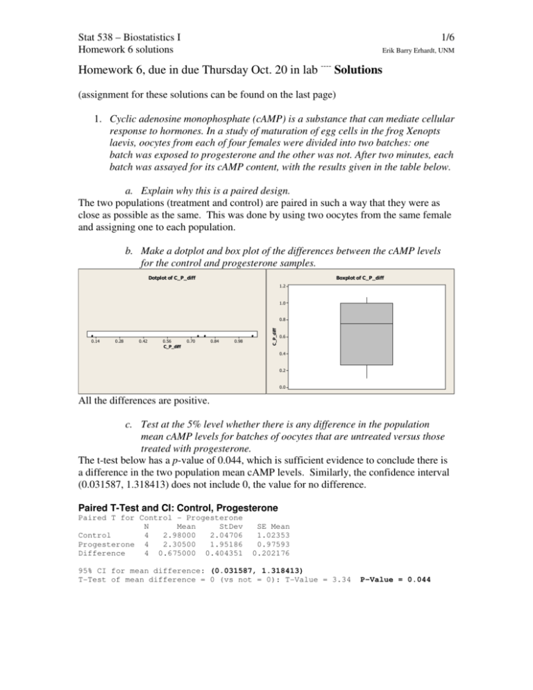
Stat 538 – Biostatistics I
Homework 6 solutions
1/6
Erik Barry Erhardt, UNM
Homework 6, due in due Thursday Oct. 20 in lab ---- Solutions
(assignment for these solutions can be found on the last page)
1. Cyclic adenosine monophosphate (cAMP) is a substance that can mediate cellular
response to hormones. In a study of maturation of egg cells in the frog Xenopts
laevis, oocytes from each of four females were divided into two batches: one
batch was exposed to progesterone and the other was not. After two minutes, each
batch was assayed for its cAMP content, with the results given in the table below.
a. Explain why this is a paired design.
The two populations (treatment and control) are paired in such a way that they were as
close as possible as the same. This was done by using two oocytes from the same female
and assigning one to each population.
b. Make a dotplot and box plot of the differences between the cAMP levels
for the control and progesterone samples.
Dotplot of C_P_diff
Boxplot of C_P_diff
1.2
1.0
0.14
0.28
0.42
0.56
C_P_diff
0.70
0.84
0.98
C_P_diff
0.8
0.6
0.4
0.2
0.0
All the differences are positive.
c. Test at the 5% level whether there is any difference in the population
mean cAMP levels for batches of oocytes that are untreated versus those
treated with progesterone.
The t-test below has a p-value of 0.044, which is sufficient evidence to conclude there is
a difference in the two population mean cAMP levels. Similarly, the confidence interval
(0.031587, 1.318413) does not include 0, the value for no difference.
Paired T-Test and CI: Control, Progesterone
Paired T for Control - Progesterone
N
Mean
StDev
Control
4
2.98000
2.04706
Progesterone 4
2.30500
1.95186
Difference
4 0.675000 0.404351
SE Mean
1.02353
0.97593
0.202176
95% CI for mean difference: (0.031587, 1.318413)
T-Test of mean difference = 0 (vs not = 0): T-Value = 3.34
P-Value = 0.044
Stat 538 – Biostatistics I
Homework 6 solutions
2/6
Erik Barry Erhardt, UNM
d. Obtain and interpret a 95% CI for the difference in population mean
cAMP levels for batches of oocytes that are untreated versus those treated
with progesterone.
From above, the confidence interval (0.031587, 1.318413) contains the true population
difference in means with 95% confidence. That is, 95% of intervals constructed in this
way contain the true difference in population means. Because 0 is not included in the
interval, we conclude there is a difference in population means.
e. Discuss any statistical assumptions that you have made in carrying out the
analysis, and whether the assumptions seem reasonable.
Because these samples are extremely small (only 4 each), we are assuming the
populations are each normal. The probability plots below indicate one observation in
each sample that deviates from an otherwise straight line through the other three. The pvalues for the Anderson-Darling normality test are 0.056 and 0.013, which are both
evidence against the normality assumption. However, the sample of differences appears
reasonably normal with a p-value=0.286.
Probability Plot of Control, Progesterone, C_P_diff
Normal - 95% CI
Control
Percent
99
Progesterone
99
90
90
50
50
10
10
1
Control
Mean
2.98
StDev
2.047
N
4
AD
0.552
P-Value 0.056
1
-5
0
5
10
C_P_diff
99
-5
0
5
10
Progesterone
Mean
2.305
StDev
1.952
N
4
AD
0.749
P-Value 0.013
C _P_diff
Mean
0.675
StDev
0.4044
N
4
AD
0.334
P-Value
0.286
90
50
10
1
-1
0
1
2
f. Write a short summary to the problem.
To study the difference in cAMP content in frogs when exposed to progesterone, a
matched-pairs design was used in a sample of size 4 in each group. A hypothesis test of
whether there is a difference was performed, and while all differences were positive,
there was evidence to conclude a difference. However, probability plots indicate the
populations of the individual samples are not normal, yet our conclusions based on tiny
samples of size 4 should be made with caution.
Stat 538 – Biostatistics I
Homework 6 solutions
3/6
Erik Barry Erhardt, UNM
2. For these data, we are interested in comparing the distribution of birth weights
for males to females.
a. Using Minitab, describe the shapes, and make sure to compare the centers
and spreads for the birth weights of males and females. Do the
distributions appear to be reasonably normal with similar spreads? Does
there appear to be much of a difference in the typical birth weights for
males compared to females? Discuss briefly.
The male data are roughly normal, the female data are skewed right.
The male data are centered 400-600 grams greater based on mean and median than the
female data.
The male spread is about 25% greater in terms of standard deviation, and twice as large
in terms of Range and IQR.
There appears to be a difference since, in terms of SE, the means are roughly 4 units from
each other.
Descriptive Statistics: weight
sex
N
Mean SE Mean
0
29
3728
107
1
19 3379.2
94.3
StDev
574
411.2
Minimum
2450
2900.0
Q1
3300
3100.0
Median
3820
3220.0
Q3
4090
3420.0
Summary for weight
Maximum
5220
4270.0
Range
2770
1370.0
Summary for weight
sex_0m_1f = 0
sex_0m_1f = 1
A nderson-D arling N ormality Test
2400
3200
4000
IQR
790
320.0
0.44
0.274
A -S quared
P -V alue <
1.33
0.005
M ean
S tD ev
V ariance
S kew ness
Kurtosis
N
3728.1
573.5
328952.5
0.028986
0.768722
29
M ean
S tD ev
V ariance
S kew ness
Kurtosis
N
3379.2
411.2
169100.7
1.13950
0.08568
19
M inimum
1st Q uartile
M edian
3rd Q uartile
M aximum
4800
A nderson-D arling N ormality Test
A -S quared
P -V alue
2450.0
3300.0
3820.0
4090.0
5220.0
2400
3200
4000
M inimum
1st Q uartile
M edian
3rd Q uartile
M aximum
4800
95% C onfidence Interv al for M ean
3509.9
95% C onfidence Interv al for M ean
3946.3
3181.0
95% C onfidence Interv al for M edian
3553.6
9 5 % C onfidence Inter vals
455.2
3999.9
775.7
Median
3577.4
95% C onfidence Interv al for M edian
3100.0
9 5 % C onfidence Inter vals
95% C onfidence Interv al for S tD ev
Mean
2900.0
3100.0
3220.0
3420.0
4270.0
3411.4
95% C onfidence Interv al for S tD ev
310.7
Mean
608.1
Median
3500
3600
3700
3800
3900
4000
3100
3200
3300
3400
3500
3600
b. Do a formal test at the 5% level that the population mean birth weights
are the same for males and females. Use the pooled t-test and do the test
by comparing the p-value to .05. Also, compare the result with what you
get from the Satterthwaite (Welch) test.
A pooled t-test gives a p-value=0.027, which at the 5% level causes us to reject H0 in
favor of HA, concluding the population means are different from each other. Using
nonequal variances, we have slightly stronger evidence for a difference in population
means, with a p-value=0.018.
Two-Sample T-Test and CI: weight, sex_0m_1f
Two-sample T for weight
sex_0m_1f
N Mean StDev
0
29 3728
574
1
19 3379
411
SE Mean
107
94
Difference = mu (0) - mu (1)
Estimate for difference: 348.893
95% CI for difference: (42.249, 655.537)
Stat 538 – Biostatistics I
Homework 6 solutions
T-Test of difference = 0 (vs not =): T-Value = 2.29
Both use Pooled StDev = 516.1413
4/6
Erik Barry Erhardt, UNM
P-Value = 0.027
DF = 46
P-Value = 0.018
DF = 45
Unpooled
95% CI for difference: (62.329, 635.457)
T-Test of difference = 0 (vs not =): T-Value = 2.45
c. Construct and interpret a 95% CI for the difference in population mean
birth weights between males and females.
The confidence intervals above do not contain 0. 95% of intervals constructed in this
way contain the true difference in population means.
d. Write a short summary of your analysis. Include any problems with
assumptions you might see that could affect the validity of your
conclusions.
In a test of the difference in population means between boy and girl weights, we find at a
5% significance level that there is a difference.
The sample of girl weights is not normal, and with a small sample this violates the
assumptions of the hypothesis test and confidence intervals.
e. Extra Credit: Repeat parts b and c using the Mann-Whitney test. Would
you change any conclusions using that analysis?
The test for a difference in population medians concludes a difference at a 5% level (pvalue=0.0341). The confidence interval is wider than above, and does not include 0. The
conclusion is the same.
Mann-Whitney Test and CI: weight_0, weight_1
weight_0
weight_1
N
29
19
Median
3820.0
3220.0
Point estimate for ETA1-ETA2 is 430.0
95.0 Percent CI for ETA1-ETA2 is (20.1,699.9)
W = 811.5
Test of ETA1 = ETA2 vs ETA1 not = ETA2 is significant at 0.0341
The test is significant at 0.0340 (adjusted for ties)
Stat 538 – Biostatistics I
Homework 6 solutions
Stat 538: Biostatistics I Homework 6, due Thursday Oct. 20 in lab
1. Cyclic adenosine monophosphate (cAMP) is a substance that can
mediate cellular response to hormones. In a study of maturation of egg
cells in the frog Xenopts laevis, oocytes from each of four females
were divided into two batches: one batch was exposed to progesterone
and the other was not. After two minutes, each batch was assayed for
its cAMP content, with the results given in the table below.
Frog
1
2
3
4
cAMP (pmol/oocyte)
Control
Progesterone
6.01
5.23
2.28
1.21
1.51
1.40
2.12
1.38
Use Minitab for this problem.
a.
Explain why this is a paired design.
b. Make a dotplot and box plot of the differences between the cAMP
levels for the control and progesterone samples.
c. Test at the 5% level whether there is any difference in the
population mean cAMP levels for batches of oocytes that are untreated
versus those treated with progesterone.
d. Obtain and interpret a 95% CI for the difference in population
mean cAMP levels for batches of oocytes that are untreated versus
those treated with progesterone.
e. Discuss any statistical assumptions that you have made in carrying
out the analysis, and whether the assumptions seem reasonable.
f. Write a short summary to the problem.
2. These data were used in HW 3 (and appear again below). Do all the
calculations in Minitab.
The following data were collected from 48 women who were at least 40
years old when they gave birth to their first child. The data concern
the gestation period of that pregnancy, and related variables on the
child and mother.
The columns are, from left to right:
1) ID
2) The child's gestation period, in weeks
3) Sex of the child (0=Male, 1=Female)
4) Birth Weight of child, in grams
5) Number of cigarettes smoked per day (on average) by the mother
6) Height of mother in cm
7) Weight of mother in kilograms at first prenatal visit
8) Weight of mother in kilograms at final prenatal visit
For these data, we are interested in comparing the distribution of
birth weights for males to females.
a. Using Minitab, describe the shapes, and make sure to compare the
centers and spreads for the birth weights of males and females. Do
the distributions appear to be reasonably normal with similar spreads?
Does there appear to be much of a difference in the typical birth
weights for males compared to females? Discuss briefly.
b. Do a formal test at the 5% level that the population mean birth
weights are the same for males and females. Use the pooled t-test and
do the test by comparing the p-value to .05. Also, compare the result
with what you get from the Satterthwaite (Welch) test.
c. Construct and interpret a 95% CI for the difference in population
5/6
Erik Barry Erhardt, UNM
Stat 538 – Biostatistics I
Homework 6 solutions
6/6
Erik Barry Erhardt, UNM
mean birth weights between males and females.
d. Write a short summary of your analysis. Include any problems with
assumptions you might see that could affect the validity of your
conclusions.
Extra Credit: Repeat parts b and c using the Mann-Whitney test.
Would you change any conclusions using that analysis?
DATA
---01 36
02 38
03 38
04 38
05 39
06 39
07 39
08 39
09 39
10 39
11 39
12 39
13 40
14 40
15 40
16 40
17 40
18 40
19 40
20 40
21 40
22 40
23 40
24 40
25 40
26 40
27 40
28 40
29 40
30 40
31 40
32 40
33 41
34 41
35 41
36 41
37 41
38 41
39 41
40 41
41 41
42 41
43 41
44 41
45 41
46 41
47 43
48 43
0
0
0
1
0
0
0
0
1
1
1
1
0
0
0
0
0
0
0
0
0
0
0
0
1
1
1
1
1
1
1
1
0
0
0
0
0
0
0
0
0
0
1
1
1
1
1
1
3300
3300
4100
2900
2820
3040
4120
4200
3100
3330
3410
3420
2450
2885
3235
3320
3600
3720
3720
3820
3840
3880
3960
4465
2980
3040
3060
3100
3120
3205
3220
4100
3100
3720
3720
3900
3990
4050
4080
4100
4460
5220
3300
3400
4000
4030
3220
4270
0
60
20
10
0
0
0
0
0
0
0
0
20
0
0
0
0
0
0
0
0
0
0
0
0
0
20
0
0
0
0
40
0
0
20
0
0
0
0
0
20
0
40
0
0
0
0
0
160.0
167.6
167.6
163.9
161.3
158.8
160.0
174.0
171.5
160.0
165.1
162.6
167.6
167.7
170.2
165.1
165.1
165.0
172.7
175.3
167.0
156.2
157.5
157.5
160.0
162.0
157.5
170.2
160.3
172.7
170.0
167.0
168.9
170.2
170.2
167.0
165.1
167.6
162.6
165.1
165.1
157.5
162.6
172.7
165.1
166.0
166.4
162.6
67.3
52.7
64.2
72.7
50.0
49.1
57.7
68.0
67.3
74.0
55.9
52.3
61.4
60.0
50.0
63.6
53.2
57.7
61.4
60.8
60.5
57.3
52.7
51.4
47.7
49.0
61.0
55.5
56.8
58.2
64.6
67.0
61.4
57.7
57.7
68.0
52.3
61.0
59.1
60.5
56.8
56.8
74.1
71.4
90.0
63.0
60.9
54.5
82.7
76.0
79.6
95.8
63.3
61.5
73.5
86.8
85.6
90.5
70.7
66.0
72.5
78.6
65.5
80.2
68.7
74.4
80.0
78.1
83.9
73.7
68.2
66.4
55.2
60.3
75.0
64.6
75.4
75.5
86.0
85.0
69.2
67.7
80.5
85.4
71.2
78.5
83.1
86.5
88.0
68.2
89.7
87.8
100.8
95.3
72.0
70.3