These notes essentially correspond to chapter 15 of the text.
This chapter deals with various rules of thumb and pricing practices that can be used by …rms who
produce multiple products or operate in multiple markets.
1
1.1
Markup pricing
Markup on price
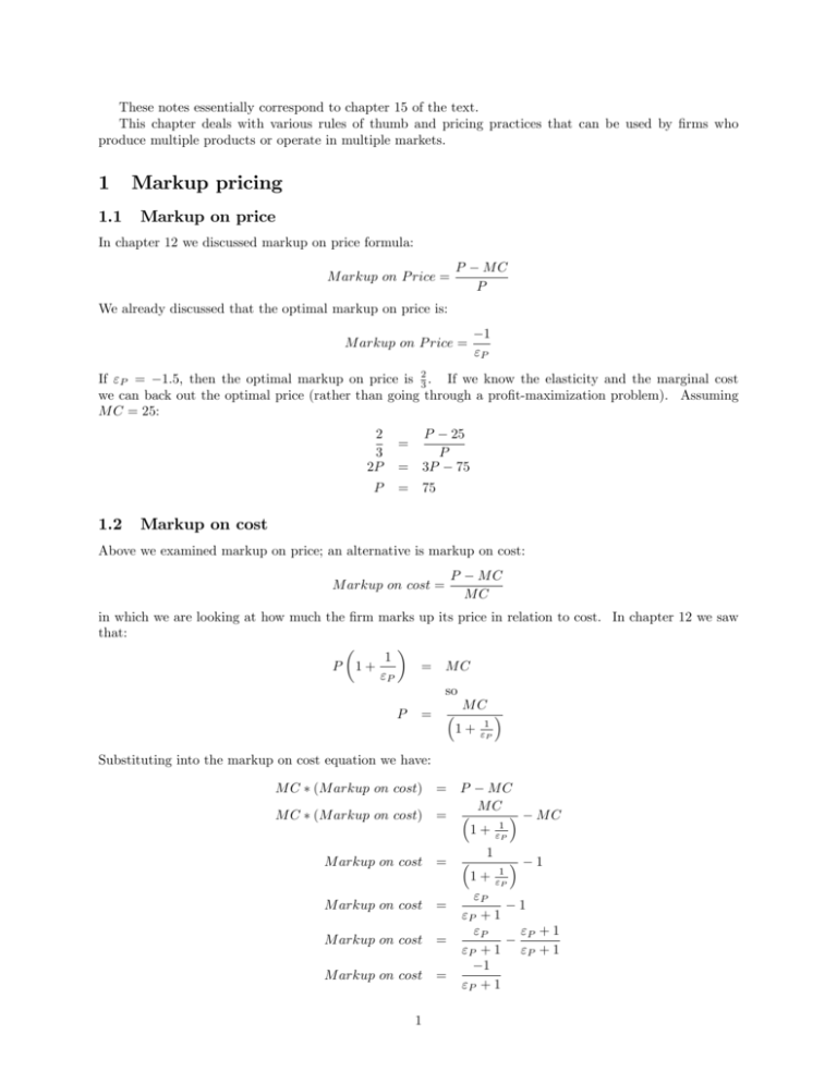
In chapter 12 we discussed markup on price formula:
M arkup on P rice =
P
MC
P
We already discussed that the optimal markup on price is:
M arkup on P rice =
1
"P
If "P = 1:5, then the optimal markup on price is 32 . If we know the elasticity and the marginal cost
we can back out the optimal price (rather than going through a pro…t-maximization problem). Assuming
M C = 25:
2
3
2P
P
1.2
P
=
25
P
= 3P
= 75
75
Markup on cost
Above we examined markup on price; an alternative is markup on cost:
P
M arkup on cost =
MC
MC
in which we are looking at how much the …rm marks up its price in relation to cost. In chapter 12 we saw
that:
P
1+
1
"P
= MC
so
P
MC
=
1+
1
"P
Substituting into the markup on cost equation we have:
MC
(M arkup on cost)
= P
MC
(M arkup on cost)
=
MC
MC
1+
M arkup on cost =
M arkup on cost =
M arkup on cost =
M arkup on cost =
1
1
1
"P
MC
1
1 + "1P
"P
1
"P + 1
"P
"P + 1
"P + 1 "P + 1
1
"P + 1
Thus, if we know the price elasticity of demand, we can determine the optimal markup on cost. If "P = 1:5,
then the optimal markup on cost is 2 or 200%. So if the cost of our item was $25, then we would need to
…nd the price such that:
2
75
P
=
25
25
= P
Note that both markup formulas are giving the same optimal price (assuming the same elasticity and marginal
cost).
2
Price discrimination
When …rms use price discrimination, they charge di¤erent prices to di¤erent groups of customers. We will
discuss the three main categories of price discrimination. Keep in mind that while the word "discrimination"
typically has a negative connotation (at least in the U.S.), price discrimination is not always bad and may
sometimes allow a market to exist when it would not exist if only a single price were charged to all customers.
All forms of price discrimination require that at least two groups (perhaps more) of customers are identi…able
and have di¤erent elasticities for the good, and typically the …rm would like to prevent resale from one party
to another.
2.1
First degree price discrimination
In …rst degree price discrimination, it is as if the …rm knows the maximum amount each individual will pay
for each unit of the good and the …rm charges each individual that maximum price (or just a little below
the maximum price). Recall that in our discussion of monopoly, a monopolist’s marginal revenue curve was
beneath it’s demand curve because the monopolist had to charge the same price to all customers, and that
this di¤erence between society’s marginal bene…t curve (the demand curve) and the monopolist’s marginal
bene…t curve (the marginal revenue curve) led to the monopolist producing too low of a quantity. If the
monopolist could …rst-degree price discriminate, then the demand curve would become the monopolist’s
marginal bene…t curve and the monopolist would produce the e¢ cient quantity (meaning there would be
no deadweight loss in the market). In the process, the monopolist would also transfer all of the consumer
surplus into producer surplus.
First degree price discrimination is more of a theoretical construct than a practical application, because
the …rm would be required to know each individual’s demand curve to charge the optimal price. The most
prevalent area for …rst degree price discrimination to occur is in negotiated sales, such as for a car, because
each individual likely pays a di¤erent price than each other and than the sticker price for the car. It is
also possible to use auctions in an attempt to …rst degree price discriminate, though there typically is some
consumer surplus that will not be captured by the auctioneer.
2.2
Second degree price discrimination
In second degree price discrimination involves discounts for purchasers of large quantities. It is easy to see
how groups of consumers are identi…ed –the …rm simply has to look at how much each consumer purchases
and place them in the correct group. This practice can be bene…cial to the …rm because the volume of
sales made to a large purchaser can o¤set the discount given to that purchaser. The …rm may not be too
concerned with whether or not the large quantity purchaser resells to other purchasers in this instance; in
fact, it may just be part of the supply chain process (for example, Wal-Mart is able to buy in bulk from
manufacturers who do not have any, or much, direct contact with …nal consumers, and Wal-Mart resells
these products at a higher price).
2.3
Third degree price discrimination
Third degree price discrimination is probably the most common form of price discrimination. Discounts for
senior citizens, lower prices for matinee (daytime) movie showings, discounts for early in the week (Monday2
Wednesday) dining out, and di¤erences in airline ‡ight tickets for business travelers and vacationers are
just some examples of third degree price discrimination. In each instance, consider how the "groups" are
identi…ed: senior citizens are identi…ed by age, people going to the movies during the day and those dining out
early in the week are identi…ed by when they are purchasing the good, and business travelers and vacationers
are (usually) identi…ed by the length of their trips. Resale in most of these instances is easily preventable
because the good has to be consumed when purchased.
2.3.1
Price discrimination example
Suppose that college students are willing to pay $10 to see a movie, and that seniors are willing to pay $5
(we will assume that there are no seniors who are college students for this example). Also assume that the
…rm can sell one extra ticket to the movie at zero MC (meaning that the MC for the …rm is a ‡at line at
zero) and that the …rm has no …xed costs, so that T R = . We will look at 3 policies: charging everyone
$10, charging everyone $5, and charging college students $10 and seniors $5 (price-discrimination). The
table below shows the pro…t from each group:
Pricing
10 college students 20 seniors Total
All $5
$50
$100
$150
All $10
$100
$0
$100
$10 College, $5 Seniors $100
$100
$200
The demand curve for movie tickets, based upon the patrons values, is also displayed below:
Price 10
8
6
4
2
0
0
10
20
30
Quantity
If the …rm charges one price to all consumers, it will maximize pro…t by charging a price of $5. This will
leave the college students with $50 of consumer surplus. However, the …rm can earn more money by price
discriminating and charging the college students $10 and the seniors $5. Thus, the …rm takes the consumer
surplus away from the college students, transferring the surplus to its own pro…t. Notice that this market
was fully e¢ cient even when a single price was charged, as the movie theater was selling a quantity of 30
tickets when it priced at $5. In this example, price discrimination allows for a transfer of consumer surplus
to producer surplus (or pro…t because there are no costs in this example).
2.3.2
Another simple example
Keep the same parameters from above, only now there are only 5 seniors instead of 20. The table becomes:
Pricing
10 college students 5 seniors Total
All $5
$50
$25
$75
All $10
$100
$0
$100
$10 College, $5 Seniors $100
$25
$125
The demand curve for the tickets is now:
3
Price 10
8
6
4
2
0
0
5
10
15
20
Quantity
The pro…t-maximizing single price in this example is $10. Note that this excludes the seniors, which
leads to a deadweight loss of $25. However, if the …rm can price discriminate, then it will be able to sell
the 5 additional tickets to the seniors, which will increase e¢ ciency (while at the same time increasing the
…rm’s own pro…ts). So in this example the ability to price discriminate actually increases the e¢ ciency in
the market.
2.3.3
Multi-market price discrimination (mathematically)
The typical method the …rm uses to price discriminate is similar to the method used above – break the
consumers into 2 or more groups and then charge the consumer a price based upon the group into which he
falls. Suppose that we have two groups, seniors and college students. College students have the inverse
demand function: P (Q) = 204 5Q and seniors have the inverse demand function P (Q) = 152 2Q.
Suppose that the marginal cost per unit is constant at $4, or M C = 4 and that the T C = 4Q. If the
monopolist can perfectly separate the two groups then it should act as a monopolist in both markets, and
set the pro…t-maximizing single-price in EACH market. For the college students:
M C (college) = 4
204
10Q = 4
200 = 10Q
20 = Q
So the price for the college students is: P (20) = 204
104 20 = 2080 from the college students.
For the seniors:
5 (20) = 104. The …rm earns total revenue of
M C (seniors) = 4
152
4Q = 4
148 = 4Q
37 = Q
The price for the seniors is: P (37) = 152
from the seniors.
2 (37) = 78. The …rm earns total revenue of 37 78 = 2886
4
The …rm’s total cost is T C = 4Q = 4 (37 + 20) = 228. Its pro…t is then: 2886 + 2080 228 = 4738. If
the …rm were to set one price in this market, it would set a price around $85. It would sell about the same
number of units, 57, but the …rm’s pro…t would only be 4631 as opposed to the 4738 above.
You should note that this type of analysis to …nd the pro…t-maximizing price only works when the
marginal costs are constant. When the marginal costs are not constant, then one must sum the two demand
curves and …nd the marginal revenue curve for this summed demand curve, and then …nd where M R = M C.
Two-part pricing1
3
With two-part pricing, a …rm charges a lump sum fee to the consumer and then charges a per-use fee. Sam’s
Club is one example of two-part pricing: consumers pay an annual membership fee, and then they have to
pay for the goods they purchase at the store. A gym membership could also be viewed as two-part pricing,
with the monthly membership fee being the lump sum payment and then any additional services (personal
training, coaching, etc.) being an additional payment beyond the membership fee. Again, the idea is that
the …rm will use this two-part pricing system to capture more of the consumer surplus (and possibly expand
production). Similar to price discrimination, the …rm must know consumer’s demand and be able to prevent
resale among consumers.
3.1
Identical consumers
Consider the case where all consumers have the same demand curve. Recall that a monopolist will not produce the e¢ cient amount of output, where e¢ cient is de…ned as the quantity where marginal cost intersects
the demand curve. Consider a typical consumer who has the demand function:
P (Q) = 80
Q
and a monopolist who has T C = 10Q. We will compare (1) the pro…t from charging the optimal single
price, (2) the pro…t from charging the optimal two-part price, and (3) the pro…t from charging a suboptimal
two-part price.
3.1.1
Optimal single price
The optimal single price is found by setting up the monopolist’s pro…t function and solving for the optimal
quantity:
= (80 Q) Q 10Q
@
= 80 2Q 10
@Q
0 = 70 2Q
Q = 35
When Q = 35, we have P = 55, and the monopolist’s optimal pro…t is:
=
=
=
3.1.2
55 35
45 35
1575
10 35
Optimal two-part price
The optimal two-part price, in the case of identical consumers, is to charge a …xed amount equal to the
entire consumer surplus and then charge a per-unit price equal to marginal cost. In this problem, because
of the constant marginal cost, the entire consumer surplus is the area of the right triangle given by (80 10)
(this is the y-intercept minus the marginal cost of 10) and the output when P = M C (we know M C = 10,
1 The
example here is from Perlo¤, Je¤rey. (2004). Microeconomics. 3 rd edition. Pearson Addison Wesley.
5
so when P = 10 we have Q = 70). The area of the triangle is 12 base height = 21 70 70 = 2450 in this
instance. So the monopolist should charge the consumer a …xed fee of $2450 and then sell the consumer
each unit of output at the level of marginal cost, so P = M C = 10. Note that the monopolist makes no
pro…t on each individual unit sold, as all of the pro…t is from the …xed fee of $2450. Note that this pro…t is
greater than the $1575 that the monopolist made from charging the optimal single per-unit price.
3.1.3
Suboptimal two-part price
Suppose that the monopolist now decides that it does not like making zero pro…t on each unit sold, and that
it decides to charge a price above its marginal cost of 10. Suppose the monopolist decides to charge $20.
Now, the consumer surplus in this market is still the area of a right triangle, but it is a right triangle with
height 60 (the intercept of 80 minus the price of 20 being charged), and a quantity sold of 60 as well (because
P (Q) = 80 Q, so when P = 20, Q = 60). We still have 12 base height = 12 60 60 = 1800. So the
optimal …xed fee, if the monopolist wishes to charge P = $20, is $1800. Clearly this amount is less than
the $2450 the monopolist earned in pro…t from the optimal …xed fee, but the monopolist also makes $10
per-unit on each unit sold when its price is $20. However, it only sells 60 units, so it makes $600 from the
per-unit sales. When added to the $1800 …xed fee, the monopolist only makes $2400 from this consumer,
which is less than the $2450 from the optimal two-part price.
3.2
Nonidentical consumers
Now consider a case with two representative consumers who have di¤erent demand curves. If the monopolist
knows each individual’s demand curve, and can prevent resale of the item, then the monopolist will maximize
pro…t by charging each consumer type a di¤erent …xed fee. Let one consumer have the demand curve from
above:
P (Q1 ) = 80 Q1
while a second consumer has the following demand curve:
P (Q2 ) = 100
Q2
We know that the optimal two-part price for the …rst consumer type is to charge $2450 as a …xed fee and
then $10 per unit. For the second type the optimal …xed fee would be 21 90 90 = 4050 and the per-unit
price would be $10. So the monopolist’s pro…t if it knows each individual demand curve is $6500.
3.2.1
Single lump sum fee and optimal pricing
Suppose the monpolist knows the demand curves but must charge the same fee and per-unit price to each
consumer (perhaps there are some legal restrictions). The monopolist will want to choose a lump sum fee
equal to the consumer surplus of one of the two types. If it charges a lump sum fee equal to the potential
consumer surplus of the second consumer type, then it will only sell to that type (the fee will be too expensive
for the …rst consumer type because that type does not value the good that much) and so we know that the
optimal fee would be $4050 and the optimal per-unit price would be $10.
Now consider a lump see fee being charged equal to the potential consumer surplus of the …rst type. We
know that if only the …rst type is in the market the optimal lump sum fee is $2450 and the optimal per-unit
price is $10. Because there are two types of consumers the consumer would receive $4900 in payments from
the two types, which is better than the $4050 it would receive from charging a lump sum fee equal to the
consumer surplus of the second type. The question is, can the …rm do better by lowering its lump sum fee
and charging a higher per-unit price?
Consider what the …rm’s pro…t is. The …rm will receive the lump sum fee from each type of consumer,
and then it will sell units to each type of consumer. The monopolist’s pro…t function is then:
= 2 CS1 + (P
Q1
C
6
Q1 ) + (P
Q2
C
Q2 )
where CS1 is the potential consumer surplus to the …rst consumer type and C is the marginal cost. The
potential consumer surplus to the …rst type is given by:
CS1
=
CS1
=
CS1
=
1
(80
2
1
(80
2
1
(80
2
P ) Q1
P ) (80
P)
2
P)
Recall that the potential consumer surplus is just the area of the triangle under the demand curve but above
the price. Now we have:
=
=
1
2
(80 P ) + (P Q1 C Q1 ) + (P
2
2
(80 P ) + (P C) (Q1 + Q2 )
2
Q2
C
Q2 )
Substituting in for Q1 and Q2 we have:
=
=
(80
(80
2
C) (80
2
C) (180
P ) + (P
P ) + (P
P + 100
P)
2P )
Now we can just di¤erentiate with respect to P , set the derivative equal to zero, and solve for the optimal
P:
@
= 2 (80 P ) ( 1) + (180
@P
0 =
160 + 2P + 180 2P
0 = 20 2P + 2C
P = 10 + C
2P ) + (P
C) ( 2)
2P + 2C
Because C = 10, we know that P = 20. We also know that the lump sum fee is:
CS1
=
CS1
=
CS1
=
1
(80
2
1 2
60
2
1800
2
P)
What is the pro…t to the …rm for setting the optimal lump sum fee and per-unit price? The …rm receives
$1800 from each consumer type so that is $3600 in lump sum fees. The …rm is also pricing above marginal
cost (which in this example is the same as average cost), so the …rm will receive $10 in pro…t from each
per-unit sale. At a price of $20, the …rm sells 60 units to the type 1 consumer, and sells 80 units to the
type 2 consumer. So there is an additional $1400 in pro…t from per-unit sales, meaning the …rm has a total
pro…t of $3600 + $1400 = $5000. Note that this pro…t is more than the pro…t the …rm earns from setting a
lump sum amount of $2450 and charging $10 per-unit (pro…t in that case was $4900).
4
Multiple product pricing
If a …rm produces products that are not interrelated in the …nal market (the cross-price elasticity between
the two goods is zero) and do not use the same production facilities, then the goods can be analyzed
separately from the …rm’s point of view. The …rm would choose the optimal production quantity based on
the M R = M C rule for each good and the …rm’s pro…t would be maximized.
However, if the …rm produces products that are interrelated in either demand or production, then a
complete analysis of each individual product market would have to incorporate the impact of each product
in all markets. For instance, Kraft produces Kraft Macaroni and Cheese as well as Kool-Aid (among many
7
other items). If sales of Kraft Macaroni and Cheese impact sales of Kool-Aid, and vice versa, then a complete
analysis of the Kraft Macaroni and Cheese market needs to incorporate its impact on the Kool-Aid market.
Assuming that only these two goods are being produced, the marginal revenue for each product would be:
M RM ac
M RK
4.1
A
@T RM ac
@T RK A
@T R
=
+
@QM ac
@QM ac
@QM ac
@T R
@T RK A
@T RM ac
=
+
@QK A
@QK A
@QK A
=
=
Fixed proportions
In some instances production will occur in …xed proportions. This result could occur if the production of
a certain amount of one good leads to a speci…c amount of "waste" that can be used to produce a speci…c
amount of a second good. We will consider the case where all units of both products will be sold (there will
be no excess waste).
Consider the total cost function:
T C = 2; 000; 000 + 50Q + 0:01Q2
While we are considering markets for two goods, because these goods are produced in the same proportion
we only need to consider the cost with producing Q units. The demand for goods A and B are:
PA
PB
= 400
= 350
0:01QA
0:015QB
TR
TR
= T RA + T RB
= PA QA + PB QB
Total revenue for the …rm is given by:
We can now construct a pro…t function:
= PA QA + PB QB
=
(400
2; 000; 000 + 50Q + 0:01Q2
0:01QA ) QA + (350
2; 000; 000 + 50Q + 0:01Q2
0:015QB ) QB
Because the two goods are produced in the same proportion, we can substitute Q for QA and QB .
substitution leads to:
=
(400
= 400Q
= 700Q
0:01Q) Q + (350
0:015Q) Q
0:01Q2 + 350Q 0:015Q2
0:035Q2 2; 000; 000
This
2; 000; 000 + 50Q + 0:01Q2
2; 000; 000
50Q
0:01Q2
Di¤erentiating the pro…t function with respect to Q, setting the derivative equal to zero, and solving we
have:
@
= 700 0:07Q
@Q
0 = 700 0:07Q
Q = 10; 000
When Q = 10; 000, we have PA = $300 and PB = $200, and the …rm will earn $1; 500; 000 in pro…t.
Before concluding that the …rm has found the optimal quantity and prices we need to make sure that
the marginal revenue for each product is greater than or equal to zero. If the marginal revenue were less
8
than zero, then we would be losing revenue with the last sale of whichever product had negative marginal
revenue. In this example we have:
M RA
M RA
M RA
M RB
M RB
M RB
4.1.1
= 400
= 400
= 200
and
= 350
= 350
= 50
0:02Q
0:02 10; 000
0:03Q
0:03 10; 000
When M R < 0 for one product
Now consider the case where M RB < 0 when solving the …rm’s joint production pro…t maximization problem.
To see this, consider that the demand for product B has fallen while cost and the demand for product A
remains as above:
TC
PA
PB
= 2; 000; 000 + 50Q + 0:01Q2
= 400 0:01QA
= 290 0:02QB
Setting up the new pro…t function we have:
= PA QA + PB QB
=
(400
2; 000; 000 + 50Q + 0:01Q2
0:01QA ) QA + (290
2; 000; 000 + 50Q + 0:01Q2
0:02QB ) QB
Again, substituting in Q for QA and QB we have:
=
(400
= 400Q
= 640Q
0:01Q) Q + (290
0:02Q) Q
0:01Q2 + 290Q 0:02Q2
0:04Q2 2; 000; 000
2; 000; 000 + 50Q + 0:01Q2
2; 000; 000
50Q
0:01Q2
Di¤erentiating with respect to Q, setting the result equal to zero and solving:
@
= 640 0:08Q
@Q
0 = 640 0:08Q
Q = 8; 000
When Q = 8; 000, we have PA = $320 and PB = $130. Pro…t for the …rm will be $560; 000 if these quantities
are sold at these prices.
Looking at M RA and M RB we have:
M RA
M RA
M RA
M RB
M RB
M RB
=
=
=
400
400
$240
and
= 290
= 290
=
$30
0:02QA
0:02 8; 000
0:04QB
0:04 8; 000
Thinking about what is happening, the …rm’s marginal cost at a production level of 8; 000 is 50+0:02 8000 =
210. So when our …rm adds the marginal revenue from the last unit of goods A and B they equal $210,
9
but product B is not contributing a positive marginal revenue. This means that the …rm could do better
by looking only at product A as that is the only product making a positive contribution towards covering
marginal cost.
When the …rm focuses only on maximizing pro…t for good A we have:
A
A
A
=
(400
= 400QA
= 350QA
2; 000; 000 + 50QA + 0:01Q2A
0:01QA ) QA
0:01Q2A
0:02Q2A
2; 000; 000
2; 000; 000
50QA
0:01Q2A
Again, di¤erentiating with respect to QA , setting the result equal to zero and solving we have:
@
= 350 0:04QA
@QA
0 = 350 0:04QA
QA = 8; 750
Now, the …rm will sell all of its QA at the price $312:50. However, it also has 8; 750 units of good B. If
the …rm sells all of its units of good B then we have:
PB
PB
PB
=
=
=
290
290
115
0:02QB
0:02 8750
So the …rm’s pro…t (from both products) would be:
= 640Q 0:04Q2
= 537; 500
2; 000; 000
Note that this pro…t is lower than the pro…t we originally found when producing only 8; 000 units! However,
the …rm should NOT sell all of its units of product B. The marginal cost for product B is e¤ectively zero
because it is being produced while also producing product A. Setting marginal revenue of product B equal
to its marginal cost we …nd that:
290
M RB
0:04QB
QB
= M CB
= 0
= 7; 250
Thus, the …rm should only sell 7; 250 of its 8; 750 units of good B. We will then have PB = 145, and the
…rm’s total pro…t will be given by:
= (400 0:01QA ) QA + (290
= $582; 500
0:02QB ) QB
2; 000; 000 + 50QA + 0:01Q2A
We use QA to determine the total cost because the …rm is producing Q = QA = QB units (8,750) but is
going to withhold some units of good B. By withholding these units (or destroying them), the …rm is able to
increase the price for …rm B and actually increase its pro…t. While it seems like a lot of work to determine
the exact quantities that should be sold, the …rm is able to increase its pro…t by $22; 500.
10