Human Development Report 2013
The Rise of the South Human Progress in a Diverse World
Technical notes
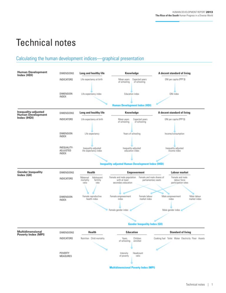
Calculating the human development indices—graphical presentation
Human Development
Index (HDI)
DIMENSIONS
Long and healthy life
INDICATORS
Life expectancy at birth
DIMENSION
INDEX
Life expectancy index
Knowledge
Mean years
of schooling
A decent standard of living
Expected years
of schooling
GNI per capita (PPP $)
Education index
GNI index
Human Development Index (HDI)
Inequality-adjusted
Human Development
Index (IHDI)
DIMENSIONS
Long and healthy life
Knowledge
INDICATORS
Life expectancy at birth
DIMENSION
INDEX
Life expectancy
Years of schooling
Income/consumption
INEQUALITYADJUSTED
INDEX
Inequality-adjusted
life expectancy index
Inequality-adjusted
education index
Inequality-adjusted
income index
Mean years
of schooling
A decent standard of living
Expected years
of schooling
GNI per capita (PPP $)
Inequality-adjusted Human Development Index (IHDI)
Gender Inequality
Index (GII)
DIMENSIONS
INDICATORS
DIMENSION
INDEX
Health
Maternal
mortality
ratio
Adolescent
fertility
rate
Female reproductive
health index
Empowerment
Labour market
Female and male population
with at least
secondary education
Female and male shares of
parliamentary seats
Female empowerment
index
Female labour
market index
Female and male
labour force
participation rates
Male empowerment
index
Female gender index
Male labour
market index
Male gender index
Gender Inequality Index (GII)
Multidimensional
Poverty Index (MPI)
DIMENSIONS
Health
INDICATORS
Nutrition Child mortality
POVERTY
MEASURES
Education
Years
of schooling
Children
enrolled
Intensity
of poverty
Headcount
ratio
Standard of living
Cooking fuel Toilet Water Electricity Floor Assets
Multidimensional Poverty Index (MPI)
Technical notes | 1
Technical note 1. Human Development Index
The Human Development Index (HDI) is a summary measure of key dimensions of human development. It measures the
average achievements in a country in three basic dimensions of
human development: a long and healthy life, access to knowledge and a decent standard of living. The HDI is the geometric
mean of normalized indices from each of these three dimensions. For a full elaboration of the method and its rationale,
see Klugman, Rodriguez and Choi (2011). This technical note
describes the steps to calculate the HDI, data sources and the
methodology used to express income.
mean of the resulting indices for the time period under consideration as the maximum. This is equivalent to applying equation 1
directly to the geometric mean of the two subcomponents.
Because each dimension index is a proxy for capabilities in the
corresponding dimension, the transformation function from
income to capabilities is likely to be concave (Anand and Sen
2000). Thus, for income the natural logarithm of the actual,
minimum and maximum values is used.
Steps to calculate the Human Development Index
The HDI is the geometric mean of the three dimension indices:
There are two steps to calculating the HDI.
(ILife 1/3 . IEducation 1/3 . IIncome 1/3).(2)
Step 1. Creating the dimension indices
Example: Ghana
Step 2. Aggregating the subindices to produce the Human
Development Index
Indicator
Minimum and maximum values (goalposts) are set in order
to transform the indicators into indices between 0 and 1. The
maximums are the highest observed values in the time series
(1980–2012). The minimum values can be appropriately conceived of as subsistence values. The minimum values are set at 20
years for life expectancy, at 0 years for both education variables
and at $100 for per capita gross national income (GNI). The low
value for income can be justified by the considerable amount of
unmeasured subsistence and nonmarket production in economies close to the minimum, not captured in the official data.
Goalposts for the Human Development Index in this Report
Indicator
Life expectancy (years)
Mean years of schooling
Expected years of schooling
Combined education index
GNI per capita (PPP $)
Observed maximum
83.6
(Japan, 2012)
13.3
(United States, 2010)
18.0
(capped at)
0.971
(New Zealand, 2010)
87,478
(Qatar, 2012)
Minimum
20.0
0
100
Having defined the minimum and maximum values, the
subindices are calculated as follows:
actual value – minimum value
.(1)
Dimension index =
maximum value – minimum value
For education, equation 1 is applied to each of the two subcomponents, then a geometric mean of the resulting indices is
created and finally, equation 1 is reapplied to the geometric mean
of the indices using 0 as the minimum and the highest geometric
2 | Technical notes
64.6
Mean years of schooling
7.0
Expected years of schooling
11.4
GNI per capita (PPP $)
1,684
Note: Values are rounded.
Life expectancy index =
64.6 – 20
= 0.701
83.6 – 20
Mean years of schooling index =
7.0 – 0
= 0.527
13.3 – 0
Expected years of schooling index =
Education index =
0
0
Value
Life expectancy at birth (years)
11.4 – 0
= 0.634
18.0 – 0
0.527 . 0.634 – 0
= 0.596
0.971 – 0
ln(1,684) – ln(100)
Income index = ln(87,478) – ln(100) = 0.417
Human Development Index =
3
0.701 . 0.596 . 0.417 = 0.558
Data sources
• Life expectancy at birth: UNDESA (2011)
• Mean years of schooling: Barro and Lee (2011) and HDRO
updates based on U
­ NESCO Institute for Statistics (2012)
data on education attainment using the methodology outlined in Barro and Lee (2010)
Human Development Report 2013
The Rise of the South Human Progress in a Diverse World
• Expected years of schooling: UNESCO Institute for Statistics (2012)
• GNI per capita: World Bank (2012a), IMF (2012), UNSD
(2012a) and UNDESA (2011)
Methodology used to express income
GNI is traditionally expressed in current monetary terms. To
make GNI comparable across time, GNI is converted from
current to constant terms by taking the value of nominal GNI
per capita in purchasing power parity (PPP) terms for the base
year (2005) and building a time series using the growth rate of
real GNI per capita, as implied by the ratio of current GNI per
capita in local currency terms to the GDP deflator.
Official PPPs are produced by the International Comparison
Program (ICP), which periodically collects thousands of prices
of matched goods and services in many countries. The last round
of this exercise refers to 2005 and covers 146 countries. The 2011
round will produce new estimates by the end of 2013. The World
Bank produces estimates for years other than the ICP benchmark based on inflation relative to the United States. Because
other international organizations—such as the World Bank and
the International Monetary Fund (IMF)—quote the base year
in terms of the ICP benchmark, the HDRO does the same.
To obtain the income value for 2012, IMF-projected GDP
growth rates (based on growth in constant terms) are applied
to the most recent GNI values. The IMF-projected growth rates
are calculated in local currency terms and constant prices rather
than in PPP terms. This avoids mixing the effects of the PPP
conversion with those of real growth of the economy.
Estimating missing values
For a small number of countries that were missing one out
of four indicators, the HDRO estimated the missing value
using cross-country regression models. The details of the
models used are available at http://hdr.undp.org/en/statistics/
understanding/issues/.
In this Report, the PPP conversion rates were estimated for
Cuba and Occupied Palestinian Territory; expected years of
schooling were estimated for Haiti, Liberia, Federated States
of Micronesia, Palau, Papua New Guinea, Sierra Leone, South
Africa, Tanzania, Turkmenistan, Zambia and Zimbabwe; and
mean years of schooling were estimated for Antigua and Barbuda, Bahamas, Cape Verde, Eritrea, Grenada, Kiribati, St. Kitts
and Nevis, St. Lucia, St. Vincent and the Grenadines, Solomon
Islands and Vanuatu. The total number of countries with an
HDI value calculated for 2012 remains 187.
Technical note 2. Inequality-adjusted Human Development Index
The Inequality-adjusted Human Development Index (IHDI)
adjusts the Human Development Index (HDI) for inequality
in the distribution of each dimension across the population. It
is based on a distribution-sensitive class of composite indices
proposed by Foster, Lopez-Calva and Szekely (2005), which
draws on the Atkinson (1970) family of inequality measures. It
is computed as a geometric mean of geometric means, calculated
across the population for each dimension separately (for details,
see Alkire and Foster 2010).
The IHDI accounts for inequalities in HDI dimensions by
“discounting” each dimension’s average value according to its
level of inequality. The IHDI equals the HDI when there is
no inequality across people but falls further below the HDI as
inequality rises. In this sense, the IHDI is the actual level of
human development (taking into account inequality), while
the HDI can be viewed as an index of the “potential” human
development that could be achieved if there was no inequality.
The “loss” in potential human development due to inequality is
the difference between the HDI and the IHDI and is expressed
as a percentage.
Data sources
Since the HDI relies on country-level aggregates such as national accounts for income, the IHDI must draw on alternative
sources of data to obtain insights into the distribution. The
distributions have different units—life expectancy is distributed across a hypothetical cohort, while years of schooling and
income are distributed across individuals.
Inequality in the distribution of HDI dimensions is estimated for:
• Life expectancy, using data from abridged life tables provided by UNDESA (2011). This distribution is grouped in age
intervals (0–1, 1–5, 5–10, ... , 85+), with the mortality rates
and average age at death specified for each interval.
• Mean years of schooling, using household survey data harmonized in international databases, including the Luxembourg Income Study, Eurostat’s European Union Survey of
Income and Living Conditions, the World Bank’s International Income Distribution Database, the United Nations
Children’s Fund’s Multiple Indicators Cluster Survey, ICF
Technical notes | 3
Macro’s Demographic and Health Survey and the United
Nations University’s World Income Inequality Database.
• Disposable household income or consumption per capita
using the above listed databases and household surveys­—or
for a few countries, income imputed based on an asset index
matching methodology using household survey asset indices
(Harttgen and Vollmer 2011).
A full account of data sources used for estimating inequality
in 2012 is available at http://hdr.undp.org/en/statistics/ihdi/.
Steps to calculate the Inequality-adjusted Human
Development Index
There are three steps to calculating the IHDI.
Step 1. Measuring inequality in the dimensions of the Human
Development Index
The IHDI draws on the Atkinson (1970) family of inequality measures and sets the aversion parameter ε equal to 1.1 In
this case the inequality measure is A = 1 – g/µ, where g is the
geometric mean and µ is the arithmetic mean of the distribution. This can be written as:
Ax = 1 –
n
X1 …Xn
– (1)
X
where {X1, …, Xn} denotes the underlying distribution in the
dimensions of interest. A x is obtained for each variable (life
expectancy, mean years of schooling and disposable income or
consumption per capita).2
The geometric mean in equation 1 does not allow zero values. For mean years of schooling one year is added to all valid
observations to compute the inequality. Income per capita
outliers—extremely high incomes as well as negative and zero
incomes—were dealt with by truncating the top 0.5 percentile
of the distribution to reduce the influence of extremely high
incomes and by replacing the negative and zero incomes with
the minimum value of the bottom 0.5 percentile of the distribution of positive incomes. Sensitivity analysis of the IHDI is
given in Kovacevic (2010).
Step 2. Adjusting the dimension indices for inequality
–
The mean achievement in an HDI dimension, X , is adjusted for
inequality as follows:
–
X . (1 – Ax) = n X1 …Xn .
4 | Technical notes
Thus the geometric mean represents the arithmetic mean
reduced by the inequality in distribution.
The inequality-adjusted dimension indices are obtained from
the HDI dimension indices, Ix, by multiplying them by (1 – Ax),
where Ax, defined by equation 1, is the corresponding Atkinson
measure:
I x* = (1 – Ax) . Ix .
*
The inequality-adjusted income index, I Income
, is actually an
adjusted index of the unlogged income values, IIncome*. This enables the IHDI to account for the full effect of income inequality.
Step 3. Combining the dimension indices to calculate the
Inequality-adjusted Human Development Index
The IHDI is the geometric mean of the three dimension indices adjusted for inequality. First, the IHDI that includes the
unlogged income index (IHDI*) is calculated:
IHDI* =
3
3
* . I*
. I*
ILife
=
Education Income
(1– ALife) . ILife . (1– AEducation) . IEducation . (1– AIncome) . IIncome*
.
The HDI based on unlogged income index (HDI*) is then
calculated:
HDI* = 3 ILife . IEducation . IIncome* .
The percentage loss in the HDI* due to in­equalities in each
dimension is calculated as:
Loss = 1 –
IHDI*
3
= 1 – (1–ALife) . (1–AEducation) . (1–AIncome) .
HDI*
Assuming that the percentage loss due to inequality in
income distribution is the same for both average income and its
logarithm, the IHDI is then calculated as:
IHDI =
IHDI* .
HDI =
HDI*
3
(1–ALife) . (1–AEducation) . (1–AIncome) . HDI .
Notes on methodology and caveats
The IHDI is based on the Atkinson index, which satisfies
subgroup consistency. This ensures that improvements or deteriorations in the distribution of human development within a
Human Development Report 2013
The Rise of the South Human Progress in a Diverse World
certain group of society (while human development remains
constant in the other groups) will be reflected in changes in
the overall measure of human development. This index is also
path independent, which means that the order in which data
are aggregated across individuals, or groups of individuals, and
across dimensions yields the same result—so there is no need to
rely on a particular sequence or a single data source. This allows
estimation for a large number of countries.
The main disadvantage is that the IHDI is not association
sensitive, so it does not capture overlapping inequalities.
To make the measure association sensitive, all the data
for each individual must be available from a single survey
source, which is not currently possible for a large number of
countries.
Example: Indonesia
Indicator
Indicator
Life expectancy (years)
Mean years of schooling
Expected years of schooling
Dimension Inequality
index
measurea (A1) Inequality-adjusted index
69.8
0.783
5.8
0.439
12.9
0.714
Education index
0.577
Logarithm of gross
national income
Gross national income (PPP $)
8.33
0.550
4,154
0.046
Human Development
Index
HDI with
unlogged
income
HDI
3
0.783 . 0.577 . 0.046 = 0.275
3
0.783 . 0.577 . 0.550 = 0.629
3
0.168
(1–0.168) ∙ 0.783 = 0.652
0.204
(1–0.204) ∙ 0.577 = 0.459
0.177
(1–0.177) ∙ 0.046 = 0.038
Inequality-adjusted Human
Development Index
Loss
(%)
0.652 . 0.459 . 0.038 = 0.225
100 .
1 – 0.225 / 0.275
= 18.3
(0.225 / 0.275) . 0.629 = 0.514
Note: Values are rounded.
a. Obtained from micro data: from life tables (UNDESA 2011) for life expectancy and from the World Bank’s
International Income Distribution Database for education and income distributions (the 2009 Survei Sosial
Ekonomi Nasional was used for Indonesia).
Technical note 3. Gender Inequality Index
The Gender Inequality Index (GII) reflects gender-­based
disadvantages in three d
­ imensions—reproductive health,
empowerment and the labour market—for as many countries
as data of reasonable quality allow. The index shows the loss
in potential human development due to inequality between
female and male achievements in these dimensions. It varies
between 0, where women and men fare e­ qually, and 1, where
either gender fares as poorly as possible in all measured
dimensions.
It is computed using the association-sensitive inequality measure suggested by Seth (2009). The index is based on the general
mean of general means of different orders—the first aggregation
is by the geometric mean across dimensions; these means, calculated separately for women and men, are then aggregated using
a harmonic mean across genders.
Data sources
• Maternal mortality ratio (MMR): WHO and others (2012)
• Adolescent fertility rate (AFR): UNDESA (2011)
• Share of parliamentary seats held by each sex (PR): IPU
(2012)
• Attainment at secondary and higher education (SE) levels:
Barro and Lee (2011) and ­U NESCO Institute for Statistics
(2012)
• Labour market participation rate (LFPR): ILO (2012)
Steps to calculate the Gender Inequality Index
There are five steps to calculating the GII.
Step 1. Treating zeros and extreme values
Because a geometric mean cannot be computed from a zero value,
a minimum value of 0.1% is set for all component indicators.
This implies that the maximum value for the maternal mortality
ratio is truncated at 1,000 deaths per 100,000 births and that
the female parliamentary representation of countries reporting
zero is coded as 0.1%. Truncating the maternal mortality ratio
can be justified by the normative assumption that countries with
a maternal mortality ratio exceeding 1,000 do not differ in their
inability to create conditions and support for maternal health.
And even in countries without female members of the national
parliament, women have some political influence.
Similarly, it is assumed that countries with 1–10 deaths per
100,000 live births are performing at essentially the same level and
that differences are random; thus, they are all assigned a value of 10.
Sensitivity analysis of the GII is given in Gaye and others (2010).
Step 2. Aggregating across dimensions within each gender
group, using geometric means
Aggregating across dimensions for each gender group by the
geometric mean makes the GII association sensitive (see Seth 2009).
Technical notes | 5
For women and girls, the aggregation formula is
GF =
3
10 . 1
MMR AFR
1/2
. (PR . SE )1/2 . LFPR , F
F
F
(1)
Health should not be interpreted as an average of corresponding female and male indices but as half the distance from the
norms established for the reproductive health indicators—fewer
maternal deaths and fewer adolescent pregnancies.
Step 5. Calculating the Gender Inequality Index
and for men and boys the formula is
GM = 3 1 . (PRM . SEM) 1/2 . LFPRM .
Comparing the equally distributed gender index to the reference standard yields the GII,
The rescaling by 0.1 of the maternal mortality ratio in equation 1 is needed to account for the truncation of the maternal
mortality ratio minimum at 10.
Step 3. Aggregating across gender groups, using a harmonic mean
1–
Harm (GF , GM )
.
–
GF,– M
Example: Brazil
Health
The female and male indices are aggregated by the harmonic
mean to create the equally distributed gender index
HARM (GF , GM) =
(GF)–1 + (GM)–1
2
–1
.
Male
Using the harmonic mean of geometric means within groups
captures the inequality between women and men and adjusts
for association between dimensions.
Step 4. Calculating the geometric mean of the arithmetic
means for each indicator
The reference standard for computing inequality is obtained by
aggregating female and male indices using equal weights (thus
treating the genders equally) and then aggregating the indices
across dimensions:
GF, M =
3
Health . Empowerment . LFPR
10 . 1
+ 1 /2,
MMR AFR
where Health =
Empowerment =
( PR
F
F + M
2
Labour market
Attainment at
secondary
Parliamentary and higher
representation
education
Labour market
participation rate
Maternal
mortality
ratio
Adolescent
fertility
rate
56.0
76.0
0.096
0.488
0.596
na
na
0.904
0.463
0.809
( )( )
10
56
1
+1
76
2
= 0.524
0.096 . 0.488 + 0.904 . 0.463
2
= 0.432
0.596 + 0.809
2
= 0.703
na is not applicable.
Using the above formulas, it is straightforward to obtain:
10 . 1 .
0.096 . 0.488 . 0.596
56 76
GF 0.185 = 3
GM 0.812 =
3
1 . 0.904 . 0.463 . 0.809
Harm (GF , GM ) 0.302=
1
1
1
+
2 0.185 0.812
3
– 0.546 = 0.524 . 0.432 . 0.703
GF,– M
)
. SE + PR . SE /2, and
F
M
M
LFPRF + LFPRM
LFPR =
.
2
6 | Technical notes
Female
Empowerment
GII 1 – (0.302/0.546) = 0.447.
–1
Human Development Report 2013
The Rise of the South Human Progress in a Diverse World
Technical note 4. Multidimensional Poverty Index
The Multidimensional Poverty Index (MPI) identifies multiple
deprivations at the individual level in education, health and
standard of living. It uses micro data from household surveys,
and—unlike the Inequality-adjusted Human Development
Index—all the indicators needed to construct the measure must
come from the same survey. More details can be found in Alkire
and Santos (2010).
Methodology
Each person is assigned a deprivation score according to his
or her household’s deprivations in each of the 10 component
indicators. The maximum score is 100%, with each dimension
equally weighted; thus the maximum score in each dimension
is 33.3%. The education and health dimensions have two indicators each, so each component is worth 33/2, or 16.7%. The
standard of living dimension has six indicators, so each component is worth 33.6/6, or 5.6%.
The thresholds are as follows:
• Education: having no household member who has completed
five years of schooling and having at least one school-age child
(up to grade 8) who is not attending school.
• Health: having at least one household member who is malnourished and having had one or more children die.
• Standard of living: not having electricity, not having access
to clean drinking water, not having access to adequate sanitation, using “dirty” cooking fuel (dung, wood or charcoal),
having a home with a dirt floor, and owning no car, truck or
similar motorized vehicle while owning at most one of these
assets: bicycle, motorcycle, radio, refrigerator, telephone or
television.
To identify the multidimensionally poor, the deprivation scores for each household are summed to obtain the
household deprivation, c. A cut-off of 33.3%, which is the
equivalent of one-third of the weighted indicators, is used to
distinguish between the poor and nonpoor. If c is 33.3% or
greater, that household (and everyone in it) is multidimensionally poor. Households with a deprivation score greater
than or equal to 20% but less than 33.3% are vulnerable to
or at risk of becoming multidimensionally poor. Households
with a deprivation score of 50% or higher are severely multidimensionally poor.
The MPI value is the mean of deprivation scores c (above
33.3%) for the population and can be expressed as a product of
two measures: the multidimensional headcount ratio and the
intensity (or breadth) of poverty.
The headcount ratio, H, is the proportion of the population
who are multidimensionally poor:
q
H=
n
where q is the number of people who are multidimensionally
poor and n is the total population.
The intensity of poverty, A, reflects the proportion of the
weighted component indicators in which, on average, poor
people are deprived. For poor households only (c greater than or
equal to 33.3%), the deprivation scores are summed and divided
by the total number of poor persons:
q
A=
∑1c
,
q
where c is the deprivation score that the poor experience.
The deprivation score c of a poor person can be expressed
as the sum of deprivations in each dimension j ( j = 1, 2, 3),
c = c1 + c 2 + c 3 .
The contribution of dimension j to multidimensional poverty
can be expressed as
q
(∑ 1 cj)/n
Contribj =
MPI
.
Example using hypothetical data
Household
Indicator
1
2
3
4
Household size
4
7
5
4
No one has completed five years of schooling
0
1
0
1
1/
÷ 2 or 16.7%
At least one school-age child not enrolled in school
0
1
0
0
1/
÷ 2 or 16.7%
At least one member is malnourished
0
0
1
0
1/
÷ 2 or 16.7%
One or more children have died
1
1
0
1
1/
3
÷ 2 or 16.7%
No electricity
0
1
1
1
1/
÷ 6 or 5.6%
No access to clean drinking water
0
0
1
0
1/
÷ 6 or 5.6%
No access to adequate sanitation
0
1
1
0
1/
÷ 6 or 5.6%
House has dirt floor
0
0
0
0
1/
÷ 6 or 5.6%
Household uses “dirty” cooking fuel
(dung, firewood or charcoal)
1
1
1
1
1/
÷ 6 or 5.6%
Household has no car and owns at most one of: bicycle,
motorcycle, radio, refrigerator, telephone or television
0
1
0
1
1/
÷ 6 or 5.6%
Weights
Education
3
3
Health
3
Living conditions
3
3
3
3
3
3
Results
Household deprivation score, c (sum of each
deprivation multiplied by its weight)
Is the household poor (c > 33.3%)?
22.2% 72.2% 38.9% 50.0%
No
Yes
Yes
Yes
Note: 1 indicates deprivation in the indicator; 0 indicates nondeprivation.
Technical notes | 7
Weighted deprivations in household 1:
Health:
(1 . 16.67) + (1 . 5.56) = 22.2%.
Headcount ratio (H) =
Contrib3 =
(80% of people live in poor households).
Intensity of poverty (A) =
(72.2 . 7) + (38.9 . 5) + (50.0 . 4)
= 56.3%
(7+5+4)
(the average poor person is deprived in 56.3% of the weighted
indicators).
MPI = H . A = 0.8 . 0.563 = 0.450.
Contribution of deprivation in:
8 | Technical notes
/ 45.0 = 29.6%
5.56 . 7 . 4 + 5.56 . 4 . 3
4+7+5+4
/ 45.0 = 37.1%
Calculating the contribution of each dimension to multi­
dimensional poverty provides information that can be useful
for revealing a country’s configuration of deprivations and can
help with policy targeting.
Notes
1 The inequality aversion parameter affects the degree to which lower achievements are emphasized and
higher achievements are de-emphasized.
2 Ax is estimated from survey data using the survey weights,
Âx = 1 – X 1w … X nw , where ∑1n wi = 1.
∑1n wi Xi
1
Education:
16.67 . 7 . 2 + 16.67 . 4
4+7+5+4
16.67 . 7 . 5 + 16.67 . 4
4+7+5+4
Living conditions:
7+5+4
= 0.800
4+7+5+4
Contrib1 =
Contrib 2 =
/ 45.0 = 33.3%
n
However, for simplicity and without loss of generality, equation 1 is referred to as the Atkinson
measure.