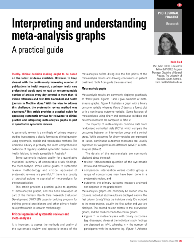
Interpreting and understanding
meta-analysis graphs
PROFESSIONAL
PRACTICE
Research
A practical guide
Ideally, clinical decision making ought to be based
on the latest evidence available. However, to keep
abreast with the continuously increasing number of
publications in health research, a primary health care
professional would need to read an unsurmountable
number of articles every day covered in more than 13
million references and over 4800 biomedical and health
journals in Medline alone.1 With the view to address
this challenge, the systematic review method was
developed.2 This article provides a practical guide for
appraising systematic reviews for relevance to clinical
practice and interpreting meta-analysis graphs as part
of quantitative systematic reviews.
A systematic review is a synthesis of primary research
studies investigating a clearly formulated clinical question
using systematic, explicit and reproducible methods. The
Cochrane Library is probably the most comprehensive
collection of regularly updated systematic reviews in the
health field and is freely accessible in Australia.3
Some systematic reviews qualify for a quantitative
statistical summary of comparable study findings,
the meta-analysis. While useful guides to systematic
review methodology and critical appraisal of
systematic reviews are plentiful, 4–6 there is a paucity
of practical guides to appraisal of meta-analysis for
the nonstatistician.
This article provides a practical guide to appraisal
of meta-analysis graphs, and has been developed as
part of the Primary Health Care Research Evaluation
Development (PHCRED) capacity building program for
training general practitioners and other primary health
care professionals in research methodology.
Critical appraisal of systematic reviews and
meta-analyses
It is important to assess the methods and quality of
the systematic review and appropriateness of the
meta-analysis before diving into the fine points of the
meta-analysis results and drawing conclusions on patient
treatment. Table 1 can guide the assessment.
Karin Ried
PhD, MSc, GDPH, is Research
Fellow & PHCRED Program
Manager, Discipline of General
Practice, The University of
Adelaide, South Australia.
karin.ried@adelaide.edu.au
Meta-analysis graphs
Meta-analysis results are commonly displayed graphically
as ‘forest plots’. Figures 1 and 2 give examples of metaanalysis graphs. Figure 1 illustrates a graph with a binary
outcome variable whereas Figure 2 depicts a forest plot
with a continuous outcome variable. Some features of
meta-analyses using binary and continuous variables and
outcome measures are compared in Table 2.
The majority of meta-analyses combine data from
randomised controlled trials (RCTs), which compare the
outcomes between an intervention group and a control
group. While outcomes for binary variables are expressed
as ratios, continuous outcomes measures are usually
expressed as ‘weighted mean difference (WMD)’ in metaanalyses (Table 2).
The details of the meta-analysis are commonly
displayed above the graph:
•review: title/research question of the systematic
review and meta-analysis
•comparison: intervention versus control group; a
range of comparisons may have been done in a
systematic review, and
•outcome: the primary outcome measure analysed
and depicted in the graph below.
Meta-analysis graphs can principally be divided into six
columns. Individual study results are displayed in rows. The
first column (‘study’) lists the individual study IDs included
in the meta-analysis, usually the first author and year are
displayed. The second column relates to the intervention
groups, and the third column to the control groups.
•Figure 1: in meta-analyses with binary outcomes
(eg. disease/no disease) the individual study findings
are displayed as ‘n/N’, whereby: n = the number of
participants with the outcome (eg. Figure 1. Adverse
Reprinted from Australian Family Physician Vol. 35, No. 8, August 2006 635
PROFESSIONAL PRACTICE Interpreting and understanding meta-analysis graphs – a practical guide
Table 1. Assessment of systematic reviews and meta-analyses
When can a systematic review and meta-analysis give further insight into primary
study results?
• Existing studies gave disparate results
• Bigger study population (sample size) can increase power, generalisability and
precision of findings (effect estimate)
• Subgroup analyses may be possible and could generate new hypotheses
Is the meta-analysis clinically sensible?
• Did the studies summarised in the systematic review address the same research
question?
• Are the studies included in the meta-analysis of comparable quality (selection bias,
attrition rates, confounding variables)?
• Are the studies comparable (eg. population, duration/dosage of treatment)?
Will the results help in caring for my patients?
• Are the studied populations comparable to my patients?
• Are the results clinically important?
• Are all clinically important outcomes considered?
• Were benefits, harms and costs considered?
Details of review
Study IDs
N = total number in group
n = number in group with the outcome
Review: Supplementation with M in condition X
Comparison: 01 Supplement M versus placebo
Outcome: 01 Adverse effects
Study
Intervention group
n/N
Control group
n/N
effects) in the intervention (column 2) or
control group (column 3), and N = the total
number of participants in the intervention
(column 2) or control group (column 3)
•Figure 2: in meta-analyses with continuous
outcome variables (eg. fasting blood
glucose level) the individual study findings
are given as ‘N’ and ‘mean (SD)', whereby
N = the total number of participants in the
intervention (column 2) or control group
(column 3), and mean SD = the arithmetic
mean and standard deviation (SD) of the
outcome measure in either the intervention
(column 2) or control group (column 3).
The fourth column visually displays the
study results. The line in the middle is called
‘the line of no effect’, which has the value of
either 1 in case of a binary outcome variable
(eg. odds ratio (OR) or relative risk [RR]), or 0
Outcome effect measure
Shown graphically and numerically
Fixed effect model used for meta-analysis
Influence of studies on
overall meta-analysis
Relative risk (fixed)
95% CI
Weight
(%)
Relative risk (fixed)
95% CI
Study A
1/141
2/142
17.8
0.50 [0.05, 5.49]
Study B
7/27
9/29
77.7
0.84 [0.36, 1.93]
Study C
1/100
0/100
4.5
3.00 [0.12, 72.77]
Total (95% CI)
268
271
100.0
0.87 [0.41, 1.87]
Total events: 9 (supplement M), 11 (control)
Overall effect
Test for heterogeneity Chi-square=0.79 df=2 p=0.67 I2=0.0%
Test for overall effect z=0.35 p=0.7
p value indicating level of
statistical significance
Heterogeneity (I2) = diversity
between studies
Figure 1. Meta-analysis of binary outcome measure
636 Reprinted from Australian Family Physician Vol. 35, No. 8, August 2006
0.01 0.1 1
Favours intervention
10
100
Favours control
Scale of treatment effect
Line of no effect
Interpreting and understanding meta-analysis graphs – a practical guide PROFESSIONAL PRACTICE
Details of review
Study IDs
N = total number in group
Mean (standard deviation) of outcome
Review: Medicines for condition X
Comparison: 01 Medicine Z versus placebo
Outcome: 01 Fasting blood glucose levels (mmol/L)
Study
Intervention group
N mean (SD)
Outcome effect measure
Shown graphically and numerically
Fixed effect model used for meta-analysis
Influence of studies on
overall meta-analysis
Control group
N mean (SD) Weighted mean difference
(fixed) 95% CI
Weight
(%)
WMD (fixed)
95% CI
Study A
34 9.77 (2.93)
34 10.29 (3.43)
27.5
–0.52 [–2.04, 1.00]
Study B
36 8.40 (1.90)
36 8.90 (3.00)
46.9
–0.50 [–1.66, 0.66]
Study C
30 10.26 (2.96)
30 12.09 (3.24)
25.6
–1.83 [–3.40, –0.26]
Total (95% CI)
100
100
100.0
–0.85 [–1.64, –0.05]
Overall effect
Test for heterogeneity Chi-square=2.03 df=2 p=0.36 I2=1.4%
Test for overall effect z=2.09 p=0.04
p value indicating level ofstatistical
significance
–4.0 –2.0 0
Favours intervention
Heterogeneity (I2) = diversity
between studies
2.0
4.0
Favours control
Scale of treatment effect
Line of no effect
Figure 2. Meta-analysis of continuous outcome measures
in case of a continuous outcome variable (eg.
WMD). There is no difference between the
intervention and the control group, if OR or RR
= 1 or WMD = 0.
The boxes are situated in line with the
outcome value of the individual studies,
also called the effect estimates (eg. OR, RR
or WMD). The value axis is at the bottom of
the graph. The size of the box is directly
related to the 'weighting' of the study in the
meta-analysis.
The horizontal lines (whiskers) through
the boxes depict the length of the confidence
intervals (CI). The longer the lines, the wider the
CI, the less precise the study results. Arrows
indicate that the CI is wider than there is space
in the graph.
The weight (in %) in the fifth column
indicates the weighting or influence of
the study on the overall results of the metaanalysis of all included studies. The higher
the percentage weight, the bigger the box,
the more influence the study has on the
overall results. The influence or ‘weight’ of
a study on the overall results is determined
by the study’s sample size and the precision
of the study results provided as a CI. In
general, the bigger the sample size and the
narrower the CI, the greater the weight of
the study.
The sixth column gives the numerical results
for each study (eg. OR or RR and 95% CI) which
are identical to the graphical display in the
fourth column.
The diamond in the last row of the graph
illustrates the overall result of the meta-
analysis. The middle of the diamond sits
on the value for the overall effect estimate (eg.
OR, RR or WMD) and the width of the diamond
depicts the width of the overall CI. The overall
numerical results are given in column six.
The total number of participants in the
intervention groups (column 2) and the control
groups (column 3) is also summarised in the
same row.
If the diamond doesn’t cross the ‘line of
no effect’, the calculated difference between
the intervention and control groups can
be considered as statistically significant.
Numerically, the CI does not include 1 for binary
outcome variables, measured as OR or RR; the
CI does not include 0 for continuous outcome
variables, measured as WMD.
Statistical significance of the overall result
Reprinted from Australian Family Physician Vol. 35, No. 8, August 2006 637
PROFESSIONAL PRACTICE Interpreting and understanding meta-analysis graphs – a practical guide
Table 2. Comparison of meta-analyses of either binary or continuous variables and outcome effect measures
Examples for variables
Binary
Continuous
Yes/no, disease/no disease, alive/deadHeight, weight, blood pressure, serum
cholesterol, walking speed
Ratios, often RR or OR
Difference between means, often WMD
1
0
Outcome effect measure
Line of no effect
Treatment scale
a) If outcome effect measure is adverse Favours intervention on left hand side
(eg. disease present, weight gain) or
of treatment scale (ratio <1)
b) if decreased outcome effect measure is desirable (eg. lowered blood
pressure)
Favours intervention on left hand side of
treatment scale (WMD <0)
Treatment scale
c) If outcome effect measure is desirable
Favours intervention on right hand
(eg. stopped smoking, increased side of treatment scale (ratio >1)
walking speed)
Favours intervention on right hand side of
treatment scale (WMD >0)
is also expressed with the probability value (p
value) in the 'test for overall effect'. Commonly,
the result is regarded as statistically significant
if p<0.05.
It is important to always check the details
on the value axis at the bottom of the graph,
as the orientation of the outcome values is
not standardised. Some graphs display the
intervention to the left side of the ‘line of no
effect’, some to the right side (Table 2). Also,
one needs to be aware if the meta-analysis
deals with binary or continuous variables. In
case of binary variables, effect values are always
greater than 0; in case of continuous variables,
values can be negative or positive.
The heterogeneity test
At the bottom of the graph on the left hand
side, the number of interest is the I2 value. I2
was only recently developed and introduced
as the preferable and more reliable test for
heterogeneity. 7 I 2 ranges between 0 and
100%. Heterogeneity measures the variability
between studies, in other words it gives
an indication how comparable studies in
the meta-analysis are. A useful visual guide
to assess heterogeneity is to check the
overlap of the CIs, ie. the horizontal lines or
whiskers in the meta-analysis graph. Studies
are regarded as homogeneous if CIs of all
studies overlap.
Assessing inter- and intra-study variation
or comparability of studies is important for
638 Reprinted from Australian Family Physician Vol. 35, No. 8, August 2006
the best choice of meta-analysis technique or
model. Generally, one can choose between two
models of meta-analysis, the 'fixed' and the
'random effect' models. If I2<=25%, studies
are regarded homogeneous and the fixed effect
model of meta-analysis can generally be used.
If I2>=75% then heterogeneity is very high, and
one should use a random effect model for metaanalysis.
Fixed and random effect models
Generally, a fixed effect model concentrates
solely on the selected studies included in
the meta-analysis, whereas a random effects
model takes into account that there might
be other studies unpublished, overlooked
in the systematic literature search, or to
be undertaken in the future which weren’t
included in the meta-analysis at hand. 8
Therefore, when the research question in
the meta-analysis is whether treatment has
produced an effect in the set of homogeneous
studies analysed, then the fixed effects model
is the appropriate one.9
Choosing the right model for analysis is
particularly important if binar y outcome
variables are used, as fixed and random
effects models give different results. In case
of continuous variables, the results of metaanalyses using fixed or random models are
often identical.8
Conflict of interest: none declared.
Acknowledgments
The author would like to thank Dr Steve Bunker
for comments on the manuscript. The Primary Health
Care Research Evaluation Development Program
is funded by the Australian Department of Health
and Ageing.
References
1. National Library of Medicine (NLM) Fact Sheet.
Bibliographic Services Division, 2005. Available at www.
nlm.nih.gov/pubs/factsheets/bsd.html.
2. Chalmers I, Hedges LV, Cooper H. A brief history of
research synthesis. Eval Health Prof 2002;25:12–37.
3. The Cochrane Library. Available at www.thecochranelibrary.com.
4. Greenhalgh T. How to read a paper. Papers that
summarise other papers (systematic reviews ad metaanalyses). BMJ 1997;315:672–5.
5. Jackson N. Systematic reviews of health promotion
and public health interventions. The Cochrane Health
Promotion and Public Health Field. Victorian Health
Promotion Foundation, 2005. Available at www.vichealth.
vic.gov.au/cochrane.
6. Hill A, Spittlehouse C. What is critical appraisal?
Including: ten questions to help you make sense of a
systematic review. Hayward Medical Communications,
2001. Available at www.evidence-based-medicine.co.uk.
7. Higgins JPT, Thompson SG, Deeks JJ, Altman DG.
Measuring inconsistency in meta-analyses. BMJ
2003;237:557–60.
8. Fleiss JL. The statistical basis of meta-analysis.
Statistical Methods in Medical Research 1993;2:121–45.
9. Bailey KR. Inter-study differences: how should they influence the interpretation and analysis of results? Statistics
in Medicine 1987;6:351–8.
CORRESPONDENCE email: afp@racgp.org.au