Using Your TI-83/84 Calculator: Binomial Probability Distributions
Elementary Statistics
Dr. Laura Schultz
This handout describes how to use the binompdf command to work with binomial probability
distributions. It also describes how to find the mean and standard deviation for all discrete
probability distributions (including binomial probability distributions) and how to generate a
probability histogram. Consider the following:
People with type O-negative blood are said to be “universal donors.” About 7% of the
U.S. population has this blood type. Suppose that 45 people show up at a blood drive.
Let x = the number of universal donors among a random group of 45 people.
The binompdf command
Let’s begin by finding the probability that none of the 45 donors have type O-negative blood.
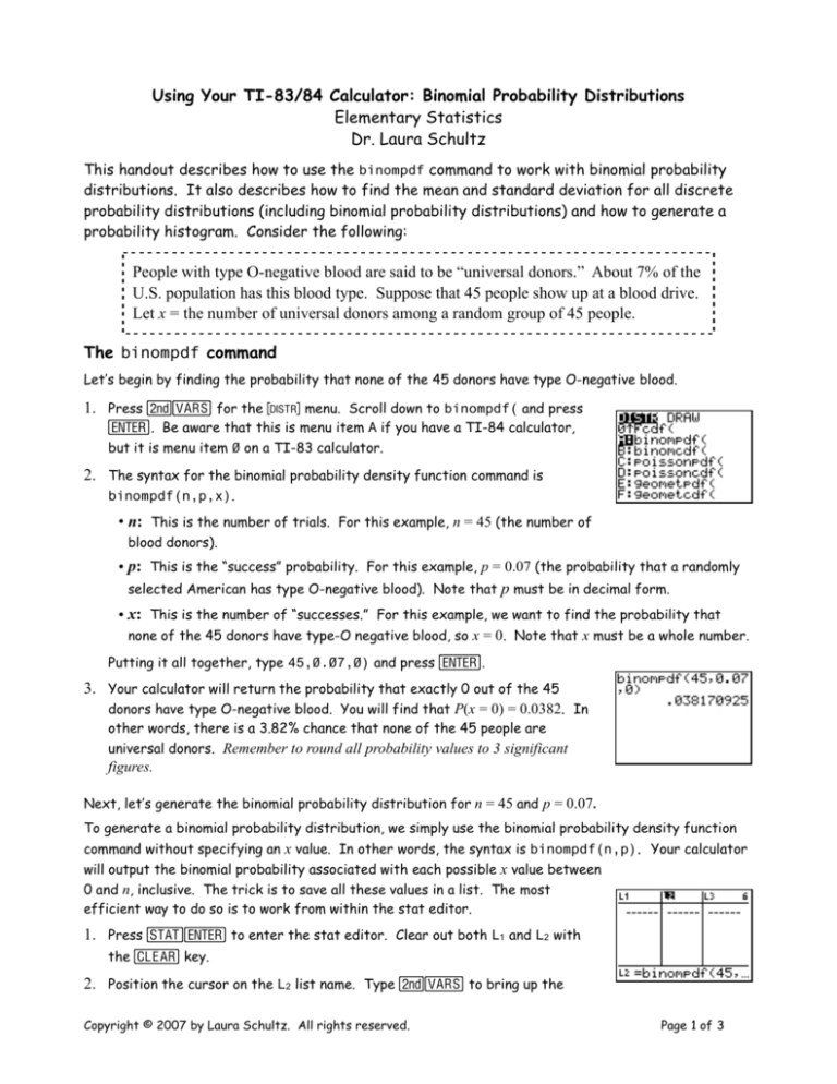
1. Press `v for the = menu. Scroll down to binompdf( and press
e. Be aware that this is menu item A if you have a TI-84 calculator,
but it is menu item 0 on a TI-83 calculator.
2. The syntax for the binomial probability density function command is
binompdf(n,p,x).
• n: This is the number of trials. For this example, n = 45 (the number of
blood donors).
• p: This is the “success” probability. For this example, p = 0.07 (the probability that a randomly
selected American has type O-negative blood). Note that p must be in decimal form.
• x: This is the number of “successes.” For this example, we want to find the probability that
none of the 45 donors have type-O negative blood, so x = 0. Note that x must be a whole number.
Putting it all together, type 45,0.07,0) and press e.
3. Your calculator will return the probability that exactly 0 out of the 45
donors have type O-negative blood. You will find that P(x = 0) = 0.0382. In
other words, there is a 3.82% chance that none of the 45 people are
universal donors. Remember to round all probability values to 3 significant
figures.
Next, let’s generate the binomial probability distribution for n = 45 and p = 0.07.
To generate a binomial probability distribution, we simply use the binomial probability density function
command without specifying an x value. In other words, the syntax is binompdf(n,p). Your calculator
will output the binomial probability associated with each possible x value between
0 and n, inclusive. The trick is to save all these values in a list. The most
efficient way to do so is to work from within the stat editor.
1. Press Se to enter the stat editor. Clear out both L1 and L2 with
the C key.
2. Position the cursor on the L2 list name. Type `v to bring up the
Copyright © 2007 by Laura Schultz. All rights reserved.
Page 1 of 3
= menu. Select binompdf( and press e.
3. You will be returned to the stat editor. Finish off the command by typing
45,0.07) and then press e.
4. Your calculator will fill up L2 with the probabilities for 0 ≤ x ≤ n successes.
5. We kept L1 empty because it is useful to indicate the x value that
corresponds to each probability value stored in L2. You could go through and
type in each x value manually, but it is often easier to generate these values
automatically. Highlight L1 and press `S to bring up the 9 menu.
6. Use the right arrow key to scroll to the OPS menu. Select 5:seq( and press
e.
7. You will be brought back to the stat editor. Complete the command by
typing X,X,0,45) and press e. (Note: Press a= to type an
“X.”) The general syntax for this command is seq(X,X,0,n).
8. Your calculator will fill L1 with the whole numbers from 0 to 45.
9. Together, L1 and L2 comprise the binomial probability distribution for n = 45
and p = 0.07. Use the ; and : keys to scroll through all the entries in L1
and L2.
Working with a binomial probability distribution
1. Let’s use the distribution we just generated to find the probability that at least one of the 45
donors has type O-negative blood. The tedious approach would be to add up P(x = 1) + P(x = 2) + P(x
= 3) +. . .+ P(x = 45). Don’t! Instead, take advantage of the fact that the complement of “at least
one” is “none.” Thus, P(1 ≤ x ≤ 45) = 1 - P(x = 0) = 1 - 0.0381709250 = 0.962. Remember to hold off
rounding to 3 significant figures until the end.
2. Next, let’s find the probability that no more than three of the donors have type O-negative blood.
To do so, we need to find P(x = 0) + P(x = 1) + P(x = 2) + P(x = 3). You could write down the
corresponding probabilities from L2 and then add them up.
3. Alternatively, we can use the sum command and specify the range of items in
L2 that we wish to add up. The key is to remember that the first item in
the list, L2(1), corresponds to P(x = 0); that is, the row number corresponds
to x + 1. Press `S for the 9 menu and scroll right for the MATH
menu. Scroll down to 5:sum( and press e.
4. The syntax for the sum command is sum(list,start,end). For this
example, type `2,1,4) and press e. This command tells
your calculator to sum the contents of rows 1 through 4 in L2. We find that
P(x ≤ 3) = 0.613. In other words, there is a 61.3% chance that no more than
three of the 45 donors have type O-negative blood.
Copyright © 2007 by Laura Schultz. All rights reserved.
Page 2 of 3
How to find μ and σ for a discrete probability distribution
1. What is the expected number (E) of universal donors
!out of the 45 people who show up at the blood
[x · P (x)] . For a binomial probability
E
=
µ
=
drive? For all discrete random variables,
distribution, E = μ = np. For this example, E = (45)(0.07) = 3.15 (round to 3.2). We can find both μ
and σ for a binomial probability distribution (or any other type of discrete
probability distribution) by using the 1-Var Stats command.
2. Press S and scroll right to the CALC menu. Press e to select 1:1Var Stats. Type `1,`2 and press e. (You must enter the
list containing the x values first, then the list containing the P(x) values.)
3. Your calculator will return the output screen shown to the right. Note that
what it calls x̄ is really μ. Rounding to one more decimal place that we
started with, we find that the expected number of universal donors out of
45 is 3.2 people, with a standard deviation of 1.7 people.
How to construct a probability histogram
1. Let’s plot a probability histogram. Press `! for the , menu.
Make sure only Plot1 is turned on. Select the histogram plot Type. The
Xlist is L1 (the list containing the x values), and Freq is L2 (the list
containing the P(x) values).
2. If you press #9, you will get an inappropriate plot. (Go ahead and see
what I mean.) We need to set the window variables. Press @. Here
are some guidelines on how to choose the proper settings:
• Xmin: Should always be 0 (the lowest possible value of x)
• Xmax: Start by using one more than the highest possible value of x in
your probability distribution (46, for this example)
• Xscl: Should always be 1
• Ymin: Should always be 0
• Ymax: Pick a value slightly higher than the largest P(x) value in L2 (Use 0.25 for this example)
• Yscl: Sets the spacing for the y-axis tick marks (0.1 is fine for this example)
• Xres: Leave it set to 1
3. Press % to generate the probability histogram. (Don’t use #!)
Then, press $ and use the > and < keys to confirm that the
histogram corresponds to the binomial probability distribution saved in L1
and L2.
4. Change the Xmax window setting to make your histogram easier to read. I
used Xmax=14 here. You’ll occasionally need to experiment with the window
settings to get a plot that captures the shape of the probability
distribution, yet is still readable.
Copyright © 2007 by Laura Schultz. All rights reserved.
Page 3 of 3