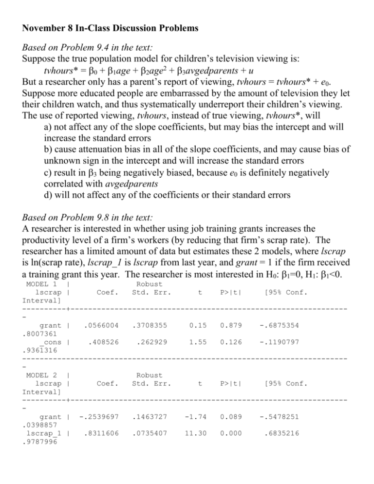
November 8 In-Class Discussion Problems
Based on Problem 9.4 in the text:
Suppose the true population model for children’s television viewing is:
tvhours* = 0 + 1age + 2age2 + 3avgedparents + u
But a researcher only has a parent’s report of viewing, tvhours = tvhours* + e0.
Suppose more educated people are embarrassed by the amount of television they let
their children watch, and thus systematically underreport their children’s viewing.
The use of reported viewing, tvhours, instead of true viewing, tvhours*, will
a) not affect any of the slope coefficients, but may bias the intercept and will
increase the standard errors
b) cause attenuation bias in all of the slope coefficients, and may cause bias of
unknown sign in the intercept and will increase the standard errors
c) result in 3 being negatively biased, because e0 is definitely negatively
correlated with avgedparents
d) will not affect any of the coefficients or their standard errors
Based on Problem 9.8 in the text:
A researcher is interested in whether using job training grants increases the
productivity level of a firm’s workers (by reducing that firm’s scrap rate). The
researcher has a limited amount of data but estimates these 2 models, where lscrap
is ln(scrap rate), lscrap_1 is lscrap from last year, and grant = 1 if the firm received
a training grant this year. The researcher is most interested in H0: 1=0, H1: 1<0.
MODEL 1 |
Robust
lscrap |
Coef.
Std. Err.
t
P>|t|
[95% Conf.
Interval]
----------+--------------------------------------------------------------grant |
.0566004
.3708355
0.15
0.879
-.6875354
.8007361
_cons |
.408526
.262929
1.55
0.126
-.1190797
.9361316
-------------------------------------------------------------------------MODEL 2 |
Robust
lscrap |
Coef.
Std. Err.
t
P>|t|
[95% Conf.
Interval]
----------+--------------------------------------------------------------grant | -.2539697
.1463727
-1.74
0.089
-.5478251
.0398857
lscrap_1 |
.8311606
.0735407
11.30
0.000
.6835216
.9787996
_cons |
.021237
.099845
0.21
0.832
-.1792103
.2216843
-------------------------------------------------------------------------. test lscrap_1=1
( 1) lscrap_1 = 1.0 F( 1,
51) =
5.27 Prob > F =
0.0258
Based on the 2 models and the F-test reported above, we can conclude
a) that the p-value for a t-statistic of (.8311-1)/.0735 = .026
b) that we should reject H0 at the 5% level
c) that there are constant determinants of the scrap rate that are correlated with
whether the firm received a training grant.
d) all of the above
Based on Example 17.1 in the text:
A researcher is estimating the probability that a married woman works as a function
of age, education, experience, number of children and other family income. The
coefficients (standard errors) on age from a linear probability model, a probit model
and a logit model are -.016 (.002), -.053 (.008) and -.088 (.015), respectively. From
this we can conclude that all else equal
a) younger women are significantly less likely to work
b) the estimated effect of age on the probability of working differs greatly
across the different models
c) a one year change in age changes the probability of working by about two
percentage points
d) all of the above
Based on Problem 17.15 in the text:
An experiment was run in which men were randomly assigned to groups, one of
which received training and one of which did not. To test whether training reduces
the probability of unemployment, the following model was estimated:
Probit estimates
Number of obs =
445
LR chi2(6)
=
8.15
Prob > chi2
= 0.2271
Log likelihood = -270.65822
Pseudo R2
= 0.0148
------------------------------------------------------------------------unem78|
dF/dx
Std. Err.
z
P>|z|
x-bar [
95% C.I.
]
--------+----------------------------------------------------------------train*|
-.107801 .043605
-2.42
0.016
.41573 -.193265 -.022337
unem74*|
.0365794 .0713216
0.51
0.613
.732584 -.103208 .176367
unem75*|
.0256093 .0671171
0.38
0.705
.649438 -.105938 .157156
age |
.0009776 .0031779
0.31
0.758
25.3708 -.005251 .007206
educ |
.0030652 .0126346
0.24
0.808
10.1955 -.021698 .027829
married*| -.0275807 .0595036
-0.46
0.648
.168539 -.144206 .089044
--------+----------------------------------------------------------------obs. P |
.3078652
pred. P |
.3049053 (at x-bar)
-------------------------------------------------------------------------(*) dF/dx is for discrete change of dummy variable from 0 to 1
z and P>|z| are the test of the underlying coefficient being 0
In a simple probit, the coefficient on train was significant and implied that the
probability of unemployment was 11 percentage points lower for those in the
training group. This model had a log likelihood of -271.5828. We can conclude
a) that the causal effect of the training program is to lower unemployment by
about 11 percentage points
b) that the simple probit is preferred to the model shown above
c) that the group assignment was truly random
d) all of the above