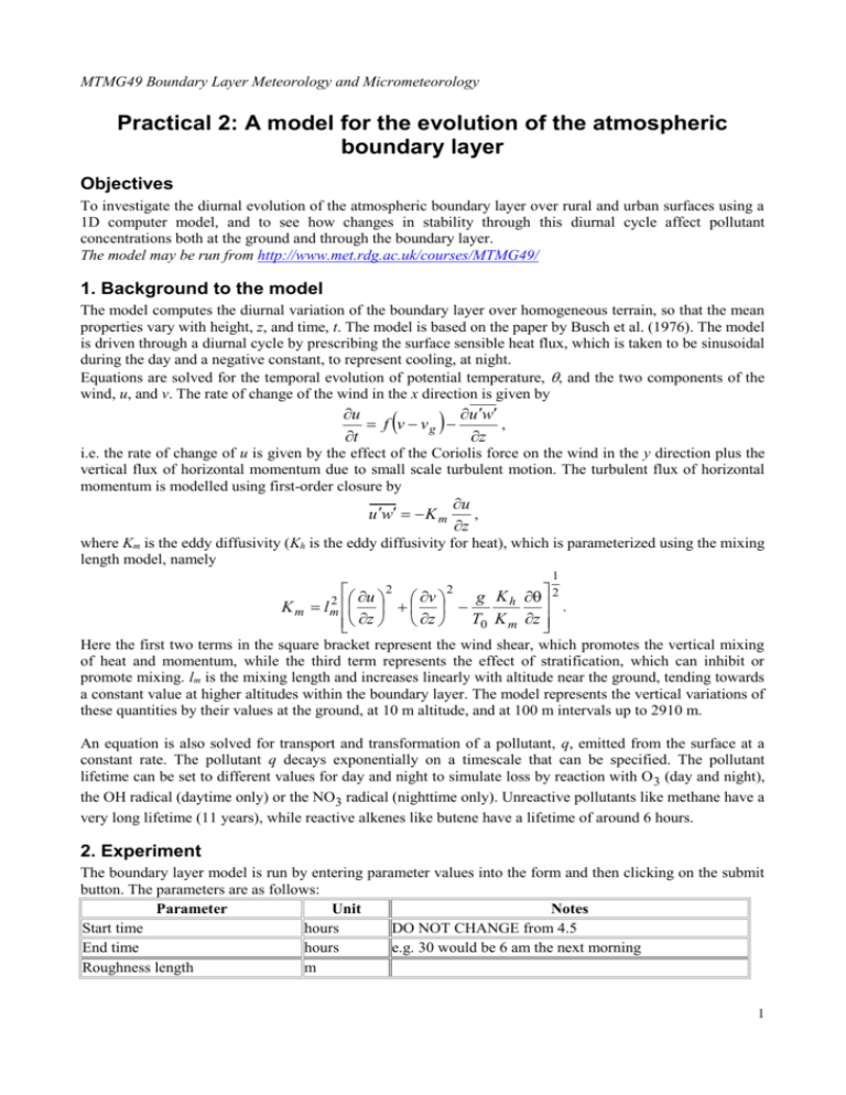
MTMG49 Boundary Layer Meteorology and Micrometeorology
Practical 2: A model for the evolution of the atmospheric
boundary layer
Objectives
To investigate the diurnal evolution of the atmospheric boundary layer over rural and urban surfaces using a
1D computer model, and to see how changes in stability through this diurnal cycle affect pollutant
concentrations both at the ground and through the boundary layer.
The model may be run from http://www.met.rdg.ac.uk/courses/MTMG49/
1. Background to the model
The model computes the diurnal variation of the boundary layer over homogeneous terrain, so that the mean
properties vary with height, z, and time, t. The model is based on the paper by Busch et al. (1976). The model
is driven through a diurnal cycle by prescribing the surface sensible heat flux, which is taken to be sinusoidal
during the day and a negative constant, to represent cooling, at night.
Equations are solved for the temporal evolution of potential temperature, , and the two components of the
wind, u, and v. The rate of change of the wind in the x direction is given by
u
u w
 f v  vg 
,
t
z


i.e. the rate of change of u is given by the effect of the Coriolis force on the wind in the y direction plus the
vertical flux of horizontal momentum due to small scale turbulent motion. The turbulent flux of horizontal
momentum is modelled using first-order closure by
u w   K m
u
,
z
where Km is the eddy diffusivity (Kh is the eddy diffusivity for heat), which is parameterized using the mixing
length model, namely
1
Km
 u  2  v  2 g K   2
h
 l m2      
 .

z

z
T
K
   
0
m z 

Here the first two terms in the square bracket represent the wind shear, which promotes the vertical mixing
of heat and momentum, while the third term represents the effect of stratification, which can inhibit or
promote mixing. lm is the mixing length and increases linearly with altitude near the ground, tending towards
a constant value at higher altitudes within the boundary layer. The model represents the vertical variations of
these quantities by their values at the ground, at 10 m altitude, and at 100 m intervals up to 2910 m.
An equation is also solved for transport and transformation of a pollutant, q, emitted from the surface at a
constant rate. The pollutant q decays exponentially on a timescale that can be specified. The pollutant
lifetime can be set to different values for day and night to simulate loss by reaction with O 3 (day and night),
the OH radical (daytime only) or the NO3 radical (nighttime only). Unreactive pollutants like methane have a
very long lifetime (11 years), while reactive alkenes like butene have a lifetime of around 6 hours.
2. Experiment
The boundary layer model is run by entering parameter values into the form and then clicking on the submit
button. The parameters are as follows:
Parameter
Unit
Notes
Start time
hours
DO NOT CHANGE from 4.5
End time
hours
e.g. 30 would be 6 am the next morning
Roughness length
m
1
MTMG49 Boundary Layer Meteorology and Micrometeorology
Model timestep
Output time interval
Geostrophic wind
s
hours
you are advised to keep this at 60 s
m s-1
N
m
Latitude
Altitude to plot wind vectors
choose from list; typically 410 m.
Maximum and minimum surface W m-2
Maximum is the maximum in daytime sinusoidal
heat fluxes
variation, minimum is the night-time minimum value
Initial temperature profile
choose from list: start with theta.dat
Pollutant lifetime (day and night) hours
Longer times for more inert chemicals
The model spins up from rest for 1.5 hours starting at 4.5 hours. Sunrise is then at 6.00 hours.
Run the model for a short integration, say a few hours, to familiarize yourself with the output. Much of the
computer time is spent processing the output data and producing plots. Make sure that you understand the
plots of the potential temperature, the wind components and the pollutant, q.
Now pick suitable input parameters for a rural boundary layer and run the model over several complete
diurnal cycles. Sketch the diurnal variation of the temperature profile and identify the different layers
(surface layer etc.). Identify the height of the boundary layer and sketch its variation with time. Note that if
more heat is input to the boundary layer in the day than is lost at night and the model is run for too many
days then the boundary layer top will reach the top of the model domain and the results will be meaningless.
Suggestions for further analysis
 The hodograph of u and v at different times (at the bottom of the output) shows the evolution of the
nocturnal jet. The height at which the hodograph is plotted can be varied. Interpret the variations that
you see through a diurnal cycle in terms of the dynamics and thermodynamics of the boundary layer.
How is this behaviour affected by latitude?
 Investigate the effect of the lifetime of the pollutant on its vertical distribution in the day and the
night. Explain physically what you find. To start it is suggested that you consider the two extremes
of a pollutant with a long and a short lifetime relative to a diurnal cycle (with the lifetimes the same
in the night and day).
 Investigate the difference between rural and urban boundary layers under the same synoptic
conditions by changing the initial parameters to reflect an urban surface (e.g. via increased surface
roughness and a minimum heat flux that is less negative). How does this affect pollution levels at the
ground and the vertical dispersion of pollution?
 Investigate the difference in pollution dispersion between summer and winter boundary layers, using
representative values for the maximum and minimum surface heat fluxes. Investigate also the role of
high and low wind speeds.
 Investigate how the Ekman wind spiral is modified by buoyancy effects by comparing the u and v
profiles between a convective boundary layer and a neutral one. A neutral daytime boundary layer
may be simulated using the constant.dat initial temperature profile and small sensible heat
fluxes (e.g. 10 W m-2 in the day and –10 W m-2 at night). Which of Ekman’s original assumptions
are compromised most in non-neutral conditions?
Reference
Busch et al. (1976), Journal of Applied Meteorology, 15, 909-919.
2