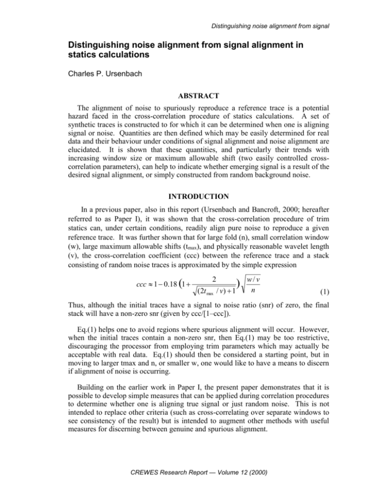
Distinguishing noise alignment from signal
Distinguishing noise alignment from signal alignment in
statics calculations
Charles P. Ursenbach
ABSTRACT
The alignment of noise to spuriously reproduce a reference trace is a potential
hazard faced in the cross-correlation procedure of statics calculations. A set of
synthetic traces is constructed to for which it can be determined when one is aligning
signal or noise. Quantities are then defined which may be easily determined for real
data and their behaviour under conditions of signal alignment and noise alignment are
elucidated. It is shown that these quantities, and particularly their trends with
increasing window size or maximum allowable shift (two easily controlled crosscorrelation parameters), can help to indicate whether emerging signal is a result of the
desired signal alignment, or simply constructed from random background noise.
INTRODUCTION
In a previous paper, also in this report (Ursenbach and Bancroft, 2000; hereafter
referred to as Paper I), it was shown that the cross-correlation procedure of trim
statics can, under certain conditions, readily align pure noise to reproduce a given
reference trace. It was further shown that for large fold (n), small correlation window
(w), large maximum allowable shifts (tmax), and physically reasonable wavelet length
(v), the cross-correlation coefficient (ccc) between the reference trace and a stack
consisting of random noise traces is approximated by the simple expression
ccc  1  0.18 (1 
2
(2t max / v)  1
)
w/ v
n
(1)
Thus, although the initial traces have a signal to noise ratio (snr) of zero, the final
stack will have a non-zero snr (given by ccc/[1–ccc]).
Eq.(1) helps one to avoid regions where spurious alignment will occur. However,
when the initial traces contain a non-zero snr, then Eq.(1) may be too restrictive,
discouraging the processor from employing trim parameters which may actually be
acceptable with real data. Eq.(1) should then be considered a starting point, but in
moving to larger tmax and n, or smaller w, one would like to have a means to discern
if alignment of noise is occurring.
Building on the earlier work in Paper I, the present paper demonstrates that it is
possible to develop simple measures that can be applied during correlation procedures
to determine whether one is aligning true signal or just random noise. This is not
intended to replace other criteria (such as cross-correlating over separate windows to
see consistency of the result) but is intended to augment other methods with useful
measures for discerning between genuine and spurious alignment.
CREWES Research Report — Volume 12 (2000)
Ursenbach
CALCULATION
The study is based on several series of calculations with synthetic traces. Each
calculation involved generating a number of reference traces, and, for each reference
trace generating n data traces to be stacked. A correlation function was calculated
between a reference trace and each one of the data traces in its stack, and, within a
given maximum allowable shift (tmax), the optimal shift was located (topt) to give the
maximum cross-correlation. The data traces were then stacked using their optimal
shifts, and the stacked trace was then cross-correlated with its reference trace, giving
a cross-correlation coefficient (ccc).
Each calculation then begins by generating the M reference traces. Each of these
is a linear combination of a “noise” component and a “signal” component
total trace = an (noise trace) + as (signal trace)
(2)
where as / an equals the signal to noise ratio of the initial data traces. The following
algorithm generated each of the two components. Each point in the .002s sample rate
trace was assigned a random number between –1 and 1. The trace was cubed in order
to thin out the number of major peaks while preserving the sign. This result was
convolved with an Ormsby wavelet of duration v. The trace was then multiplied by a
window function which has a value of unity from –w/2 to w/2, and zero elsewhere.
This defines a correlation window of duration w. Although the “signal” component
was generated randomly, it was saved for use in generation of the data traces as well.
Each reference trace was associated with a stack of n data traces. These n traces
were generated in the same fashion as the reference trace, but with two differences:
First, they possess a window size of w+2tmax to allow displacements of up to  tmax.
Second, their “signal” component, instead of being generated randomly, was obtained
by shifting the “signal” component of the reference trace, the size of the shift being
generated randomly from a Gaussian distribution of width g. In this study g has been
set equal to v for most of the calculations. The resulting shifts are thus to be
corrected by the statics procedure. The same an and as were used in both the
reference and data traces. For an = 0 we have pure signal, and for as = 0 we have pure
noise.
The output of the calculation consists of the cross-correlation coefficient (ccc)
between the stacked trace and the reference trace averaged over the M reference
traces, which will be denoted <ccc> (<…> represents an average over the M
reference traces). This well-known quantity is given explicitly as
ccc = Cstack,ref(t) / [Cstack(0)*Creference(0)]1/2
(3)
where Ci,j(t) is a time cross-correlation function, and Ci(t) is a time autocorrelation
function.
The output also includes three other quantities, which we define here. The first is
the amplitude ratio. This is the average over the M reference traces of the ratio of
zero-time autocorrelations of the stacked trace and the reference trace.
CREWES Research Report — Volume 12 (2000)
Distinguishing noise alignment from signal
amplitude ratio = <Cstack(0)/Creference(0)>
(4)
This latter quantity is useful because two traces that are simply proportional to each
other (i.e., not having the same absolute amplitude, but identical in all other respects)
will have a cross-correlation coefficient of 1. The amplitude ratio will, in such a case,
be sensitive to the differing amplitudes. For this quantity to be meaningful of course
the traces should be scaled to a common rms amplitude.
The second quantity to define is the relative shift. This is the average over the M
reference traces of the average absolute value shift of the data traces, divided by one
half of the maximum allowable shift. It may be written
relative shift = <avg(|topt|)>/(tmax/2)
(5)
where “avg(…)” represents an average over all n data traces in a stack. Dividing by
tmax/2 normalizes this quantity to unity when topt is chosen randomly from the allowed
shift interval, as is the case when random noise is being aligned. This quantity can
take on values between 0 and 2, but when tmax is much larger than the width of actual
signal statics (the Gaussian distribution, for this synthetic data), the relative shift will
tend to zero for properly aligned signal.
The third quantity is the realignment. This is an artificial quantity that can be
calculated only because we are using synthetic data. It constitutes a “back of the
book” answer to tell us whether we are aligning true signal or not. To begin we
calculate the average of the sum of the initial amount by which the true signal is
offset in creation of a data trace, and the amount by which it is shifted by the
correlation procedure. This may be written as
R = <avg(topt + t0)> / [g(2/)]
(6)
where t0 is the time shift originally applied in generating a data trace. For the initial
Gaussian distribution (topt = 0) it can readily be shown that <avg(topt + t0)> tends to
g(2/), so that the above form yields 1. For properly aligned data traces it will give
zero, and for random noise with large tmax it will tend to infinity. Thus, for
convenience in plotting we define
realignment = (R2 – 1) / (R2 + 1)
(7)
which is 0 for stacks of the initial data traces, –1 for aligned signal, and +1 for aligned
noise.
The variables that are adjusted for each calculation are the window size (w, in
seconds), the maximum allowable shift (tmax, in seconds), and the number of data
traces to be stacked (n). Other variables that we hold fixed are the number of
reference traces (M = 10), the wavelet parameters (f1 = 5, f2 = 10, f3 = 50, f4 = 70, v
= .08s), and g, the width of the normal distribution that is used for generating initial
signal offsets. g is set equal to v for most of the results in this paper, but also to 2v
for a few calculations at the end.
CREWES Research Report — Volume 12 (2000)
Ursenbach
RESULTS FOR PURE NOISE AND PURE SIGNAL
To begin we will consider cases of pure noise (as = 0) and pure signal (an = 0). In
Paper I we considered the dependence of <ccc> on n, w, tmax and v. In this paper we
will consider primarily the variation with w and tmax, as these are quantities that can
most easily be varied in normal statics calculations, and will thus most readily allow
the results obtained to be developed into practical methods. However, a few
comments about n dependence are appropriate to clarify the behaviour of the defined
quantities.
Dependence on n for random noise traces
Figures 1a-d illustrate the dependence on n of various quantities, given a selection
of values of w and tmax (tmax is the same as t in the Figure). In all cases the abscissa is
given as (w/v/n) as this was shown in Paper I to effectively organize the data when
plotting 1–<ccc>.
Figure 1. The dependence on n (the stack fold) of the cross-correlation coefficient, the
amplitude ratio, the relative shift, and the realignment (all defined in the “Calculations”
section). The data traces that have been stacked and cross-correlated to obtain this data are
constructed from pure random noise. The quantities as defined illustrate in different ways
that as n increases, noise is aligned to reproduce a reference trace.
Figure 1a displays 1–<ccc> vs. (w/v/n), where, as in Paper I, a linear approach to
the origin is apparent for large n, with plots grouped by their value of tmax. Figure 1b
shows that the amplitude ratio also decreases with n. This could be anticipated from
inspection of Figure 1 in Paper I, which shows that the amplitude of stacked data
decreases with n. This is to be expected, since the amplitude of stacked signal
increases as n, but that of stacked noise as n, so that after dividing by n to obtain the
CREWES Research Report — Volume 12 (2000)
Distinguishing noise alignment from signal
displayed stacks, the amplitude of the random stack should decrease as 1/n. Thus
the amplitude ratio as defined above should also vary as 1/n, as is approximately
observed in Figure 1b. Note that the plots in Figure 1b are grouped primarily by their
value of w, and only secondarily by tmax. Figure 1c shows that the relative shift
oscillates about 1, the value expected for random noise. Figure 1d shows that, for
small tmax, the final shifts are of a similar magnitude to the original Gaussian shifts
(realignment = 0) but that for larger tmax the shifts move away from correct
realignment (realignment>0). This assures us that the increase of <ccc> with n comes
from alignment of noise, not signal (which should be the case, as there is no signal).
Dependence on tmax for random noise traces
Figures 2a-d illustrate dependencies on tmax for various values of n and w. The
abscissa is given as 1/(2tmax/v+1) as in Paper I. Figure 2a shows 1–<ccc>
approaching linearly to the y-axis, with constant w/n plots on the same line. Solid
lines show the behaviour predicted by Eq.(1). In Figure 2b the amplitude ratio is
plotted. The ratio increases with increasing tmax. Here we see that lines of data are
grouped primarily by their value of w, and only secondarily by their value of n. The
amplitude ratio decreases with both w and n, but more strongly with the former. In
Figure 2c we see that the relative shift is essentially independent of w and n and for
tmax /v>.25 the relative shift is essentially 1. Figure 2d contains our “back of the
book” answer which, by approaching 1, confirms that noise is being aligned at large
tmax.
Figure 2. The dependence of the defined quantities (see “Calculations” section) on a function
of tmax, the maximum allowable shift. The data traces that have been stacked and crosscorrelated to obtain this data are constructed from pure random noise. The quantities as
defined illustrate in different ways that as tmax increases, noise is aligned to reproduce a
reference trace.
CREWES Research Report — Volume 12 (2000)
Ursenbach
Dependence on tmax for pure signal traces
Figures 3a-d give plots analogous to Figure 2 but for normally shifted data traces
of pure signal, and these contrast strongly with those for the random noise. In Figure
3a there is no tendency to follow the lines from Eq.(1), and values appear to depend
only on tmax. This is reasonable since the pure signal data traces are distributed about
a central point so that, for a given value of tmax, they would average to a well defined
non-zero trace that is independent of w or n. In Figure 3b the amplitude ratio initially
increases as in the random noise case, but reaches a value of 1 and levels off sharply.
The values are again independent of both w and n. In Figure 3c the relative shift
begins leveling off at 1, but then drops down to zero. The relative shifts are equal to
absolute shifts divided by tmax/2. If signal is being aligned, then the absolute shift
should become constant after a certain point. Plotting 1/tmax vs. 1/tmax should give a
parabola, and this is approximately the behaviour observed near the origin.
Figure 3. The dependence of the defined quantities (see “Calculations” section) on a function
of tmax, the maximum allowable shift. The data traces that have been stacked and crosscorrelated to obtain this data are all identical to the reference trace, but have been shifted
randomly using a Gaussian distribution of time shifts. The plots illustrate that when t max is
sufficiently large, the signal is aligned to reproduce a reference trace.
Finally, the approach of realignment to –1 in Figure 3d indicates that the signal is
being shifted back to its position in the reference trace. Note that the realignment is
essentially complete well before relative shift reaches zero.
CREWES Research Report — Volume 12 (2000)
Distinguishing noise alignment from signal
Dependence on w for random noise traces
Figures 4a-d illustrate dependencies on w for various values of n and tmax. The
abscissa is given as (w/v/n) as in Paper I.
Figure 4a shows 1–<ccc> linearly approaching the origin, with plots grouped by
the value of tmax, and solid lines showing the Eq.(1) behaviour. In Figure 4b the
amplitude ratio multiplied by (w/v/n) is plotted against (w/v/n). The reason for
multiplying the amplitude ratio before plotting is to enhance the distinction between
this plot and that which will follow for pure signal. The plots level off to a constant
for (w/v/n)>1/2, indicating that the amplitude decreases as 1/w above this point.
The plots are grouped primarily by their value of n, and only slightly by the value of
tmax. In Figure 4c we see that the relative shift clusters closely about 1.
Figure 4d indicates that the degree of realignment is essentially determined by tmax,
and is tending towards noise alignment as tmax increases.
Figure 4. The dependence of the defined quantities (see “Calculations” section) on a function
of w, the cross-correlation window. The data traces that have been stacked and crosscorrelated to obtain this data are constructed from pure random noise. The quantities
illustrate that as w decreases, noise is aligned to reproduce a reference trace.
CREWES Research Report — Volume 12 (2000)
Ursenbach
Dependence on w for pure signal traces
Again the behaviour for pure signal is very different from that of random noise, as
seen in Figure 5. In Figure 5a there is again strong deviation from Eq.(1), and values
level off at larger w, depending essentially on tmax. In Figure 5b the amplitude ratio
also apparently levels off, as multiplying it by the abscissa yields a straight line. The
plots are now grouped only by their value of tmax. Figure 5c shows that the relative
shift is about zero for small tmax, but drops to about 0.8 for larger tmax. Figure 5d
confirms that for the small tmax, the signal is slightly realigned, while for larger tmax,
the signal is completely realigned.
Figure 5. The dependence of the defined quantities (see “Calculations” section) on a function
of w, the cross-correlation window. The data traces that have been stacked and crosscorrelated to obtain this data are all identical to the reference trace, but have been shifted
randomly using a Gaussian distribution of time shifts. The plots illustrate that when tmax is
sufficiently large, the signal is aligned to reproduce a reference trace.
RESULTS FOR MIXED SIGNAL AND NOISE
In this section we ask whether the differences in behaviour described in the
previous section can be used to create a tool to discern when noise is being aligned to
mimic signal, and when true signal is being aligned. To do this we have carried out
three sets of calculations with mixed noise and signal. Each is characterized by a
particular signal-to-noise ratio (snr), with 1:3, 2:1, and 1:1 being the ratios employed.
CREWES Research Report — Volume 12 (2000)
Distinguishing noise alignment from signal
Dependence on tmax for mixed traces
Figures 6-8 illustrate the tmax dependence for systems with differing signal to noise
ratios. Figures 6a-c show remarkable similarity to Figure 2a-c, suggesting that noise
alignment is occurring for the case when the snr is 1:3, and this is confirmed by
Figure 6d.
Figures 7a,b for snr = 2:1 are similar to Figures 3a,b, but level off to different
values for large tmax. Note that the correlation actually tends to decrease slightly as
tmax increases for large tmax. This would be impossible for the cross-correlation of an
individual data trace, but although the stack depends linearly on the data traces, ccc of
the stack does not depend linearly on the ccc of individual traces, because of the
normalizing factor. So in this region ccc of individual data traces is increasing, while
that of the stack is decreasing. Continuing on, we note that Figure 7c is nearly
identical to 3c. One would assume signal alignment, and this is confirmed by Figure
7d.
Finally, turning to snr = 1:1, from Figures 8a and 8c one would conclude that the
large w plots represent signal alignment, while the small w plots appear to be
following random noise behaviour to a degree. Figure 8b is less informative.
Turning to 8d we see in fact that a divergence of behaviour based on window size
does indeed develop for large tmax. Noise vs. signal alignment is clearly sensitive to
cross-correlation parameters and not just to the snr.
One important thing to note is that the relative shift values of <1 in Figure 8c are
not sufficient to imply signal alignment. The trend is important in these tmax plots.
Figure 6. The dependence on tmax for a signal to noise ratio (snr) of 1:3. Comparison with
Figure 2 shows that the plot behaviours shown here are signatures for noise alignment.
CREWES Research Report — Volume 12 (2000)
Ursenbach
Figure 7. The dependence on tmax for a signal to noise ratio (snr) of 2:1. Comparison with
Figure 3 shows that the plot behaviours shown here are signatures for signal alignment.
Figure 8. The dependence on tmax for a signal to noise ratio (snr) of 1:1. Comparison with
Figures 6 and 7 shows in this case that different choices of cross-correlation window size can
result in either signal alignment (large window) or noise alignment (small window).
CREWES Research Report — Volume 12 (2000)
Distinguishing noise alignment from signal
Dependence on w for mixed traces
Figures 9-11 show the w dependence of the same systems as in Figures 6-8. Again
the snr = 1:3 plots in Figure 9 are remarkably similar to the random noise plots in
Figure 4. One point of difference is that the scaled amplitude appears to be linearly
increasing for the n = 64, t = 0.128s plot, typical of signal alignment behaviour. The
plots however are still closely clustered, as in Figure 4b.
Comparison of Figure 10 with Figure 5 shows a clear indication of signal
alignment by any of the three measures for snr = 2:1.
Turning to snr = 1:1, Figures 11a,b suggest that all plots are showing signal
alignment at large w, while Figure 11c suggests that signal is aligning at the larger
tmax. Looking at the answer book in Figure 11d we see that the stacks can indeed be
well aligned for tmax = .128s but that neither signal nor noise is aligned for tmax =
.032s.
Figure 9. The dependence on w for a signal to noise ratio (snr) of 1:3. Comparison with
Figure 4 shows that the plot behaviours shown here are signatures for noise alignment.
CREWES Research Report — Volume 12 (2000)
Ursenbach
Figure 10. The dependence on w for a signal to noise ratio (snr) of 2:1. Comparison with
Figure 5 shows that the plot behaviours shown here are signatures for signal alignment.
Figure 11. The dependence on w for a signal to noise ratio (snr) of 1:1. These plots illustrate
some cautionary points in use of these measures, such as the fact that the relative shift does
not necessarily need to be zero for signal to be well aligned, and conversely that signal
alignment signatures of <ccc> and [(w/v/n)*(amplitude ratio)] do not necessarily imply full
signal alignment.
CREWES Research Report — Volume 12 (2000)
Distinguishing noise alignment from signal
Dependence for larger statics
Statics analysis is generally more favourable for corrections less than v than for
corrections larger than v (Cox, 1999, Section 7.4). All of the data considered so far
has been for statics with a distribution width of v. Figures 12 and 13 display results
for g = 2v for the most favourable input data traces, SNR = 2.0.
Figure 12 should be compared with Figure 7, as their input differs only in the
value of g. In Figure 12a-c it would appear that signal is being well aligned. This is
confirmed in Figure 12d. (Note however that two extra points have been calculated at
very large tmax for w = .256, n = 16, and these appear to not be well aligned. This
may however be simply bad statistics because of the small n.) Thus alignment can
occur, even for large statics.
Figure 13 appears
only for g), but there
appear slightly more
qualitative difference
the signal is stronger.
generally similar to Figure 10 (from which it differs in input
are some slight differences as well. Both Figure 13a and 13b
typical of random noise behaviour. Thus there is no strong
from increasing g, but the tendency to align noise along with
Figure 12. This figure is analogous to Figure 7 except that the Gaussian width g of statics is
equal to 2v instead of v.
CREWES Research Report — Volume 12 (2000)
Ursenbach
Figure 13. This figure is analogous to Figure 10 except that the Gaussian width g of statics is
equal to 2v instead of v. Alignment is not as favourable for g>v.
DISCUSSION
From the above results, we conclude that to properly align signal one must have a
sufficiently large window (see Figures 10d,11d) and sufficiently large tmax (see
Figures 3d,5d,7d,8d,12d). One would like to know for certain however whether one
has selected parameters that result in noise alignment. By constructing intermediate
stacks one can calculate the cross-correlation coefficient, the amplitude ratio, and the
relative shift at several values of w and tmax. The following plots should then be
useful litmus tests to help distinguish noise alignment from signal alignment:
1. 1–<ccc> vs. 1/(2tmax /v+1): If Eq.(1) is followed, noise is being aligned. If
correlation decreases with increasing tmax, and deviates from Eq.(1), and is
independent of w/n, one is safe in continuing to increase tmax.
2. amplitude ratio vs. 1/(2tmax /v+1): If plots are grouped by w, then noise is
being aligned. If plots are independent of w and clearly level off sharply, then
signal is being aligned. This latter effect may be difficult to assign clearly.
3. relative shift vs. 1/(2tmax /v+1): If relative shift approaches zero as tmax
increases, then the signal has been aligned. If the relative shift clusters about
1, the signal has not yet been aligned, and it is possible that noise is being
aligned, even if clustering is about a number less than one.
4. 1–<ccc> vs. (w/v/n): If Eq.(1) is followed, noise is being aligned. If the plots
level off to a constant, then noise is not being aligned, but tmax is not
necessarily large enough to align the signal.
5. [(w/v/n)*(amplitude ratio)] vs. (w/v/n): If the plot levels off to a constant for
large w, and if multiple plots are grouped by n, then noise is being aligned. If
CREWES Research Report — Volume 12 (2000)
Distinguishing noise alignment from signal
the plots form separated increasing straight lines grouped by tmax, then noise is
not being aligned, but signal may or may not be fully aligned, depending on
tmax.
6. relative shift vs. (w/v/n): if the relative shift clusters about 1, the signal has
not yet been aligned, and it is possible that noise is being aligned.
Of the various quantities, <ccc> appears most suited to demonstrating explicitly
the alignment of noise (via Eq.(1)), while a plot of relative shift vs. tmax is the clearest
method for showing establishing conclusively the alignment of signal. The amplitude
ratio appears less reliable on its own, but may be useful as a corroborating indicator.
Calculation of the desired quantities (ccc, amplitude ratio, and relative shift) could
readily be implemented in existing trim statics calculations. To apply these tests to
real data one would then only need to know w and tmax (both cross-correlation
parameters), n (a property of the input data, which may also be lowered if desired),
and w (a property of the input data, which may be estimated from the frequency
content).
CONCLUSIONS
This study has defined certain quantities that may be easily calculated in the course
of a statics cross-correlation procedure and plotted against functions of w, tmax, n, and
v. These plots exhibit characteristic behaviours that can assist in establishing
protocols for safe statics calculations by avoiding spurious alignment of noise.
ACKNOWLEDGEMENTS
The author wishes to thank Dr. John Bancroft for helpful discussions and generous
support during the course of this work.
REFERENCES
Cox, M., 1999, Static Corrections for Seismic Reflection Surveys: SEG, Tulsa, OK.
Ursenbach, Charles P. and Bancroft, John C., Noise alignment in trim statics: CREWES Research
Report, Volume 12, 2000
CREWES Research Report — Volume 12 (2000)