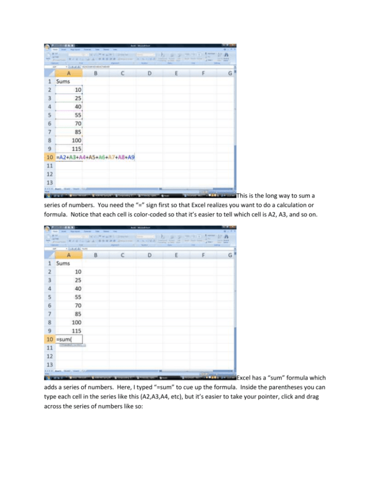
This is the long way to sum a
series of numbers. You need the “=” sign first so that Excel realizes you want to do a calculation or
formula. Notice that each cell is color-coded so that it’s easier to tell which cell is A2, A3, and so on.
Excel has a “sum” formula which
adds a series of numbers. Here, I typed “=sum” to cue up the formula. Inside the parentheses you can
type each cell in the series like this (A2,A3,A4, etc), but it’s easier to take your pointer, click and drag
across the series of numbers like so:
I started with my pointer on cell
A2, clicked and held the button down, and then dragged down through cell A9 (I call this “highlighting
the cells” or “blocking the cells out”). Excel writes A2:A9 (meaning sum up the numbers in cells A2
through A9), and then you type in the closing parenthesis. Hit “Enter” and the formula sums up the
series.
Finally, you could click in cell A10,
then click on “AutoSum” to add up the series. In Office 2007, this is in the top right hand of the “Home”
menu. In earlier versions, look for the Greek letter sigma ∑ in the tool bar. In this case the numbers add
up to 500.
Payback Period Example
Here we’ve got two investment choices – A and B – each with non-uniform net cash flows (n.c.f.).
Investment A lasts 5 years and B lasts 6 years. Our initial investment was $1000 and we want to get our
money back in 4 years or less. Which investment pays back the fastest? We have to use the payback
ratio measure:
N
i.i.
N
 n.c. f .
1
In cells B13 and C13, I have calculated the sum of the n.c.f. (the bottom
n 1
of our ratio for all six years. To calculate the N value, divide the initial investment ($1000) by the sum of
n.c.f.
The N ratio for A and B is in cells B11 and C11 respectively.
The N is less than 1 for both
investments. Payback comes earlier than six years, so sum the n.c.f. for a shorter time period.
Here, the n.c.f. for A are summed through 2 years, while the n.c.f. for B are summed through 4 years.
A’s N = 1.1, while B’s N=1. B pays
back in exactly 4 years. A pays back in a little bit longer than 2 years. Sum A’s n.c.f. through 3 years, and
N = 0.833, so option A pays back in a little longer than 2 years. Which investment is best? Both pay back
in 4 years or less, but A pays back faster, so choice A is best. Look at the total profits over the life of
each investment. B provides greater benefits – that’s a problem with payback method. It doesn’t take
into account all the benefits of an investment.
An Example of Compounding
With compounding, we’re looking for the Future Value (FV) of a dollar amount today (PV), if we take the
PV and invest it in an opportunity with a given rate of return or interest rate (r). If the interest rate is
compounded annually, that means interest is added in once per year. The formula looks like this:
FV  PV 1  r 
n
If interest is compounded more than once per year, then we have to alter the formula to incorporate
the number of compounding periods (m).
r

FV  PV 1  
 m
n *m
If interest is compounded quarterly, then m=4. If interest is compounded
monthly, then m=12.
Let’s say we have $1000, and we want to put it in a bank account that earns 5% interest, compounded
annually. How much will we have after five years?
FV = ? PV = $1000
r=0.05 or 5%
m = 1 (because we’re compounding annually)
Use a calculator to figure out the answer manually with the formula.
Here’s how we do it in Excel:
Click on the fx symbol; that brings up
the dialog box.
Click on Financial in the dropdown
box, then scroll down to FV. Double
click on FV or click once on FV and
then click OK
The FV formula dialog box appears. “Rate” means the interest rate. “Nper” refers to the total number
of periods (the number of years – N – multiplied by the number of compounding periods – m). If we had
a uniform series of payments (an annuity), we could enter the amount of the payment in the “PMT” box.
In this example, though, we just have one payment at the beginning, so our initial investment goes in
the PV box.
You could type in $1000 in the PV box, 0.05 in the Rate box and 1 in the Nper box, but I prefer to use cell
references. This way, if I want to change the PV or the Rate or the number of compounding periods, I
can make the change in the spreadsheet without having to redo the formula every time. Also, I have $
in the cell reference for Rate and for N – this is called Fixed Reference. If I had several PVs that I wanted
to use compounding on, Fixed Reference allows me to copy the formula and not have to follow all these
steps each time. Fixed Reference means that each time I copy the formula, it will still refer to the cell
with the original rate, original N, etc. Saves work later on.
Excel has one other quirk. It doesn’t realize that you are paying $1000 initially and earning interest, so
the formula will return a negative number for the answer. In order to get a positive number for the
answer, you tell Excel that you are paying $1000 initially by putting a negative sign in front of the PV.
Then Excel will return a positive answer. The FV of $1000 today, compounded annually at 5% over 1
year is $1050.
Compounding with
different numbers of compounding periods.
An Example of Discounting
Discounting takes a FV and calculates what that FV is worth today (the PV). If my uncle wants to give my
$1500 in five years, after I have graduated from college, it’s not the same as if he gave me $1500 today.
Why? Because I have to wait five years to get that $1500. If he gave me $1500 today, I could do a lot
with that. I could host a series of keg parties, or I could put a down payment on a car, or I could buy a
new rifle, etc. There’s an opportunity cost of having to wait five years; $1500 five years from now is not
worth $1500 today. Discounting accounts for that waiting period. The discounting formula looks like
this:
PV 
FV
It’s just the compounding formula after some algebra torture to solve for PV.
1  r n
With multiple compounding periods, the formula becomes:
PV 
FV
r

1  
 m
FV = $1500
example)
n*m
r=0.05 (if we had the same bank account opportunity as with our compounding
Using the PV formula – click on the fx symbol as before, go to financial, scroll down to PV and click OK.
The PV of my uncle’s
gift is $1175. By making me wait five years, he’s really only giving me $1175.29.