Case Study 28
28
Modeling Queuing Systems
Modeling Queuing Systems
Problem Description
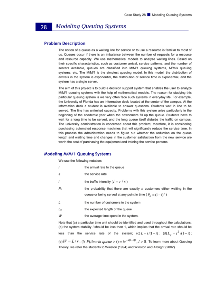
The notion of a queue as a waiting line for service or to use a resource is familiar to most of
us. Queues occur if there is an imbalance between the number of requests for a resource
and resource capacity. We use mathematical models to analyze waiting lines. Based on
their specific characteristics, such as customer arrival, service patterns, and the number of
servers available, queues are classified into M/M/1 queuing systems, M/M/s queuing
systems, etc. The M/M/1 is the simplest queuing model. In this model, the distribution of
arrivals in the system is exponential, the distribution of service time is exponential, and the
system has a single server.
The aim of this project is to build a decision support system that enables the user to analyze
M/M/1 queuing systems with the help of mathematical models. The reason for studying this
particular queuing system is we very often face such systems in everyday life. For example,
the University of Florida has an information desk located at the center of the campus. At the
information desk a student is available to answer questions. Students wait in line to be
served. The line has unlimited capacity. Problems with this system arise particularly in the
beginning of the academic year when the newcomers fill up the queue. Students have to
wait for a long time to be served, and the long queue itself disturbs the traffic on campus.
The university administration is concerned about this problem; therefore, it is considering
purchasing automated response machines that will significantly reduce the service time. In
this process the administration needs to figure out whether the reduction on the queue
length and waiting time and changes in the customer satisfaction from the new service are
worth the cost of purchasing the equipment and training the service persons.
Modeling M/M/1 Queuing Systems
We use the following notation:
r
the arrival rate to the queue
s
the service rate
i
the traffic intensity ( i
Pn
the probability that there are exactly n customers either waiting in the
 r/s)
queue or being served at any point in time ( Pn  (1  i) n )
L
the number of customers in the system
Lq
the expected length of the queue
W
the average time spent in the system.
Note that (a) a particular time unit should be identified and used throughout the calculations;
(b) the system stability i should be less than 1, which implies that the arrival rate should be
the
service
rate
of
the
system;
(c) L  i /(1  i ) ;
(d) Lq
 i 2 /(1  i ) ;
less
than
(e) W
 L / r ; (f) P(time in queue  t )  ie s(1i)t , l  0 . To learn more about Queuing
Theory, we refer the students to Winston (1994) and Winston and Albright (2002).
Case Study 28
Modeling Queuing Systems
Solution Algorithm
Step 1
Collect data about students’ arrival and service time at the information desk. Use this data to
simulate the system AS IS. To learn about how to build a simulation model in order to
replicate an M/M/1 queuing system by using Microsoft Excel, we refer the students to
Winston (1994). Collect the following statistics from the simulation: average/minimum/
maximum queue length, average waiting time in the queue, average time in the system (t),
and average utilization of the server.
Step 2
Build a simulation model considering that automated machines are used instead of a server.
To run this simulation, use the data collected about students’ arrival at the information desk
and estimates about the service time at the automated response machines. Collect the
following statistics for the new system: average/minimum/ maximum queue length, average
waiting time in the queue, average total time in the system (t new), and average utilization of
the machines.
Step 3
n
Calculate: X 
 (t
i 1
i
 t i* )
; where ti is the time spent currently in the system by student i,
n
and ti* is the time spent in the system by student i if the new system is in place. Thus, X is
the average time saved per student. Calculate the total savings per unit of time ( X * r ).
Calculate the total costs saved using the new system X * r * m , where m is the subjective
cost of having a student wait for one unit of time in the system. Calculate the cost of using
the automated response machines per unit of time (Y). One can calculate Y based on the
amortization of the machines per time unit. For the purpose of this project, one can use
straight-line amortization. To learn more about straight-line amortization, we refer the
students to Park (2003). If Y  X * r * m , we can say that the addition of the automated
machines is beneficial and the administration should implement it.
Excel Spreadsheets
1.
Build a spreadsheet that presents the arrival time of the students in the system.
2.
Build a spreadsheet that presents the service time at the information desk.
User Interface
1.
Build a welcome form.
2.
Build a data entry form. The following are suggestions for designing this form. Insert a
frame that includes two option buttons. The option buttons enable the user to select
whether to read the data from a file or enter the data manually. Include a command
button that, when clicked on, performs these actions:
a.
If the user chose to read the data from a file, a text box should appear where the
user types in the name of the file.
Case Study 28
b.
Modeling Queuing Systems
If the user chose to enter the data manually, a text box should appear where the
user types in the total number of observations Z. Once this information is
submitted, a table with dimensions Z by 2 appears. The user types in the arrival
time of each observation and the corresponding service time.
Insert two text boxes where the user can type in the purchasing cost of automated
response machines and the total number of machines to be purchased. Insert a text box
where the user can type in the cost of having a student wait for one unit of time in the
system.
3.
4.
Insert a frame titled “Simulate the M/M/1 Queuing System.” The frame includes the
following:
a.
A sub-frame titled “Simulate the Current System.” The frame includes three text
boxes where the user can type in the simulation length, the total number of
simulation runs, and the length of the warm-up period. Insert a command button
titled “Run the Simulation” that, when clicked on, runs the simulation model for the
current system (runs Step 1 of the solution algorithm), prepares the corresponding
reports, and prompts the user to open these reports.
b.
A sub-frame titled “Simulate the New System.” The frame includes three text boxes
where the user can type in the simulation length, the total number of simulation
runs, and the length of the warm-up period. Insert a command button titled “Run the
Simulation” that, when clicked on, runs the simulation model for the new system
(runs Step 2 of the solution algorithm), prepares the corresponding reports, and
prompts the user to open these reports.
c.
Insert a command button that, when clicked on, compares the two systems (runs
Step 3 of the solution algorithm) and opens Form 4, described below.
Build a form that summarizes the results from analyzing this M/M/1 queuing system.
The following are suggestions for designing this form.
a.
Insert a frame titled “Reports” that has a number of option buttons. The option
buttons enable the user to choose to open one of the summary reports described
below.
b.
Insert a frame titled “Sensitivity Analysis” that has the following: two combo boxes
to allow the user to select a distribution for the service time and the arrival of the
customer in the queue; text boxes to allow the user to enter the corresponding
parameters of arrival time and service time; a text box where the user can type in
the total number of automated response machines to be purchased. Include a
command button that, when clicked on, performs the sensitivity analysis with
respect to the selected parameter. For example, the user might be interested to
know the sensitivity of the solution with respect to service time, the number of
automated machines purchased, etc.
Design a logo for this project. Insert this logo in the forms created above. Pick a background
color and a font color for the forms created. Include the following in the forms created: record
navigation command buttons, record operations command buttons, and form operations
command buttons as needed.
Reports
1.
Report the following statistics:
a.
The average/minimum/maximum number of customers in the current system.
K T
K T
K T
k 1t 1
k 1t 1
k 1t 1
min :   ckt xkt    hkt I kt    Fkt z kt
Case Study 28
Subject to :
K
 zkt  1
Modeling Queuing Systems
b. forThe
t average/minimum/maximum
1,..., T ,
(1) number of customers in the new system.
k 1
c.
xkt  I k ,t 1  I kt  d kt
xkt  Pkt z kt
d.
e.
xkt , I kt  0
f.
z kt  {0,1}
The average/minimum/maximum waiting time in the current system.
for k  1,..., K ; t  1,..., T ,
(2)
for k  1,..., K ; t  1,..., T ,
(3)
for k  1,..., K ; t  1,..., T ,
(4)
The average/minimum/maximum waiting time in the new system.
The average/minimum/maximum queue length in the current system.
The average/minimum/maximum queue length in the new system.
for k  1,..., K ; t  1,..., T .
(5)
g.
The average/minimum/maximum time spent in the current system.
h.
The average/minimum/maximum time spent in the new system.
i.
The probability that a customer would spend more than 10 minutes in the queue in
the current system.
j.
The probability that a customer would spend more than 10 minutes in the queue in
the new system.
k.
Server utilization in the current system.
l.
Server utilization in the new system.
m. The average (waiting and service) time saved per student when using the new
system.
n.
The total (waiting and service) savings per unit of time when using the new system
( X * r ).
o.
The total costs savings per unit of time when using the new system ( X
p.
The equipment amortization per unit of time.
* r * m ).
Based on these statistics, demonstrate whether the new system is better than the
current one.
2.
Report the results from the sensitivity analysis.
Reference
Park, C., “Contemporary Engineering Economics.” Prentice Hall, 3rd Ed., 2003.
Winston, L.W., “Operations Research: Applications and Algorithms.” Duxbury Press, 3rd Ed.,
1994.
Winston, L.W., Albright, S.C., “Practical Management Science: Spreadsheet Modeling &
Applications Update,” Duxbury Press, 2002.