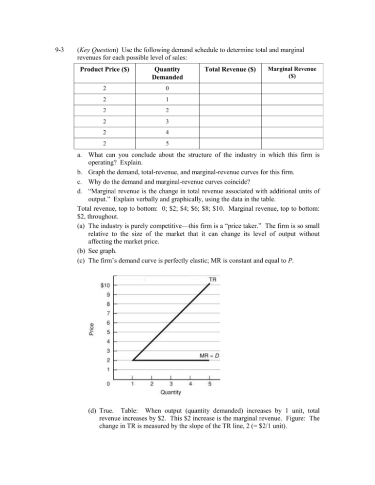
9-3
(Key Question) Use the following demand schedule to determine total and marginal
revenues for each possible level of sales:
Product Price ($)
Quantity
Demanded
2
0
2
1
2
2
2
3
2
4
2
5
Total Revenue ($)
Marginal Revenue
($)
a. What can you conclude about the structure of the industry in which this firm is
operating? Explain.
b. Graph the demand, total-revenue, and marginal-revenue curves for this firm.
c. Why do the demand and marginal-revenue curves coincide?
d. “Marginal revenue is the change in total revenue associated with additional units of
output.” Explain verbally and graphically, using the data in the table.
Total revenue, top to bottom: 0; $2; $4; $6; $8; $10. Marginal revenue, top to bottom:
$2, throughout.
(a) The industry is purely competitive—this firm is a “price taker.” The firm is so small
relative to the size of the market that it can change its level of output without
affecting the market price.
(b) See graph.
(c) The firm’s demand curve is perfectly elastic; MR is constant and equal to P.
(d) True. Table: When output (quantity demanded) increases by 1 unit, total
revenue increases by $2. This $2 increase is the marginal revenue. Figure: The
change in TR is measured by the slope of the TR line, 2 (= $2/1 unit).
9-4
(Key Question) Assume the following cost data are for a purely competitive producer:
Total
Product
Average
fixed
cost
Average
variable
cost
Average
total
cost
0
1
2
3
4
5
6
7
8
9
10
$60.00
30.00
20.00
15.00
12.00
10.00
8.57
7.50
6.67
6.00
$45.00
42.50
40.00
37.50
37.00
37.50
38.57
40.63
43.33
46.50
$105.00
72.50
60.00
52.50
49.00
47.50
47.14
48.13
50.00
52.50
Marginal
cost
$45
40
35
30
35
40
45
55
65
75
a. At a product price of $56, will this firm produce in the short run? Why or why not?
If it is preferable to produce, what will be the profit-maximizing or loss-minimizing
output? Explain. What economic profit or loss will the firm realize per unit of
output?
b. Answer the relevant questions of 4a assuming product price is $41.
c. Answer the relevant questions of 4a assuming product price is $32.
d. In the table below, complete the short-run supply schedule for the firm (columns 1
and 2) and indicate the profit or loss incurred at each output (column 3).
(1)
Price
$26
32
38
41
46
56
66
(2)
Quantity
supplied,
single firm
(3)
Profit (+)
or loss (l)
(4)
Quantity
supplied,
1500 firms
____
____
____
____
____
____
____
$____
____
____
____
____
____
____
____
____
____
____
____
____
____
e. Explain: “That segment of a competitive firm’s marginal-cost curve which lies above
its average-variable-cost curve constitutes the short-run supply curve for the firm.”
Illustrate graphically.
f. Now assume there are 1500 identical firms in this competitive industry; that is, there
are 1500 firms, each of which has the same cost data as shown here. Calculate the
industry supply schedule (column 4).
g. Suppose the market demand data for the product are as follows:
Price
$26
32
38
41
46
56
66
9-6
Total
quantity
demanded
17,000
15,000
13,500
12,000
10,500
9,500
8,000
What will be the equilibrium price? What will be the equilibrium output for the industry?
For each firm? What will profit or loss be per unit? Per firm? Will this industry expand
or contract in the long run?
(a) Yes, $56 exceeds AVC (and ATC) at the profit-maximizing output. Using the MR =
MC rule it will produce 8 units. Profits per unit = $7.87 (= $56 - $48.13); total profit
= $62.96.
(b) Yes, $41 exceeds AVC at the loss—minimizing output. Using the MR = MC rule it
will produce 6 units. Loss per unit or output is $6.50 (= $41 - $47.50). Total loss =
$39 (= 6  $6.50), which is less than its total fixed cost of $60.
(c) No, because $32 is always less than AVC. If it did produce according to the MR =
MC rule, its output would be 4—found by expanding output until MR no longer
exceeds MC. By producing 4 units, it would lose $82 [= 4 ($32 - $52.50)]. By not
producing, it would lose only its total fixed cost of $60.
(d) Column (2) data, top to bottom: 0; 0; 5; 6; 7; 8; 9, Column (3) data, top to bottom in
dollars: -60; -60; -55; -39; -8; +63; +144.
(e) The firm will not produce if P < AVC. When P > AVC, the firm will produce in the
short run at the quantity where P (= MR) is equal to its increasing MC. Therefore,
the MC curve above the AVC curve is the firm’s short-run supply curve, it shows the
quantity of output the firm will supply at each price level. See Figure 21.6 for a
graphical illustration.
(f) Column (4) data, top to bottom: 0; 0; 7,500; 9,000; 10,500; 12,000; 13,500.
(g) Equilibrium price = $46; equilibrium output = 10,500. Each firm will produce 7
units. Loss per unit = $1.14, or $8 per firm. The industry will contract in the long
run.
(Key Question) Using diagrams for both the industry and a representative firm, illustrate
competitive long-run equilibrium. Assuming constant costs, employ these diagrams to
show how (a) an increase and (b) a decrease in market demand will upset that long-run
equilibrium. Trace graphically and describe verbally the adjustment processes by which
long-run equilibrium is restored. Now rework your analysis for increasing- and
decreasing-cost industries and compare the three long-run supply curves.
See Figures 9.8 and 9.9 and their legends. See figure 9.11 for the supply curve for an
increasing cost industry. The supply curve for a decreasing cost industry is below.
9-7
(Key Question) In long-run equilibrium, P = minimum ATC = MC. Of what
significance for economic efficiency is the equality of P and minimum ATC? The
equality of P and MC? Distinguish between productive efficiency and allocative
efficiency in your answer.
The equality of P and minimum ATC means the firms is achieving productive efficiency;
it is using the most efficient technology and employing the least costly combination of
resources. The equality of P and MC means the firms is achieving allocative efficiency;
the industry is producing the right product in the right amount based on society’s
valuation of that product and other products.