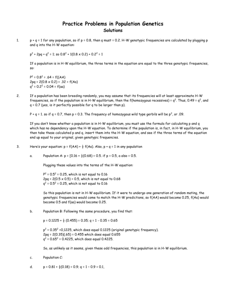
Practice Problems in Population Genetics
Solutions
1.
p + q = 1 for any population, so if p = 0.8, then q must = 0.2. H-W genotypic frequencies are calculated by plugging p
and q into the H-W equation:
p2 + 2pq + q2 = 1; so 0.82 + 1(0.8 x 0.2) + 0.22 = 1
If a population is in H-W equilibrium, the three terms in the equation are equal to the three genotypic frequencies,
so:
P2 = 0.82 = .64 = f((AA)
2pq = 2(0.8 x 0.2) = .32 = f(Aa)
q2 = 0.22 = 0.04 = f(aa)
2.
If a population has been breeding randomly, you may assume that its frequencies will at least approximate H-W
frequencies, so if the population is in H-W equilibrium, then the f(homozygous recessives) = q2. Thus, 0.49 = q2, and
q = 0.7 (yes, is it perfectly possible for q to be larger than p).
P + q = 1. so if q = 0.7, then p = 0.3. The frequency of homozygous wild type gerbils will be p 2, or .09.
If you don’t know whether a population is in H-W equilibrium, you must use the formula for calculating p and q
which has no dependency upon the H-W equation. To determine if the population is, in fact, in H-W equilibrium, you
then take these calculated p and q, insert them into the H-W equation, and see if the three terms of the equation
end up equal to your original, given genotypic frequencies.
3.
Here’s your equation: p = f(AA) + ½ f(Aa). Also, p + q = 1 in any population
a.
Population A: p = [0.16 + ½(0.68) = 0.5. if p = 0.5, a also = 0.5.
Plugging these values into the terms of the H-W equation:
P2 = 0.52 = 0.25, which is not equal to 0.16
2pq = 2(0.5 x 0.5) = 0.5, which is not equal to 0.68
q2 = 0.52 = 0.25, which is not equal to 0.16
So this population is not in H-W equilibrium. If it were to undergo one generation of random mating, the
genotypic frequencies would come to match the H-W predictions, so f(AA) would become 0.25, f(Aa) would
become 0.5 and f(aa) would become 0.25.
b.
Population B: Following the same procedure, you find that:
p = 0.1225 + ½ (0.455) = 0.35; q = 1 - 0.35 = 0.65
p2 = 0.352 =0,1225, which does equal 0.1225 (original genotypic frequency).
2pq = 2(0.35)(.65) = 0.455 which does equal 0.655
q2 = 0.652 = 0.4225, which does equal 0.4225.
So, as unlikely as it seems, given these odd frequencies, this population is in H-W equilibrium.
c.
Population C:
d.
p = 0.81 + ½(0.18) = 0.9; q = 1 – 0.9 = 0.1,
p2 = 0.92 = 0.81
2pq = 2(0.9)(0.1) = 0.18
q2 = 0.12 = 0.01
All of these equal the originally provided genotypic frequencies, so this population is in H-W equilibrium.
e.
Population D:
P = 0.04 + ½(0.6) = 0.34; q = 1 – p = 0.66
P2 = 0.342 = 0.1156
2pq = 2(0.34)(0.66) = 0.4488
q2 = 0.662 = 0.4356
These do not equal the original genotypic frequencies supplied, so this population is not in H-W equilibrium
(despite the fact that f(DD) and f(dd) look like such nice, neat squares). Should this population go through
a generation of random mating, the genotypic frequencies would come to match the predictions of the HW equation, so f(AA) would become 0.1156, f(Aa) would become 0.4488 and f(aa) would become 0.4356.
4.
This is a selection problem. Farmer Jones is completely selecting against the homozygous recessive dwarf plants by
not allowing them to contribute to upcoming generations. For selection problems, you must first calculate
q—the
amount that q will be changed by one generation of selection—then apply q to see what your new generation’s q
will be, and calculation genotypic frequencies from there.
a.
For the 2001 crop: qo2 = 0.09, so qo = 0.3
q = -(qo2)/(1 + qo) = -(0.32)/(1 + 0.3) = -.09/1.3 = -0.07 (rounded)
Note that this is a negative number, and that it is only the amount q will change, not the actual new q. To
get that we must add
q1 = qo +
q to qo (remember that q is negative, so adding it to qo will reduce the size of q).
q = 0.23
For the new generation, again assuming random mating the frequency of dwarf plants = q12 = 0.232 = 0.53
(rounded)
b.
For 1992,
q must be calculated beginning with q1, not qo. So for this year, q = -(q12)/1 + q1) = -0.043. q2 =
For 1993
q = -0.029 and q3 = 0.158
a = -0.021 and q4 = 0.137
q1 + q = 0.187
For 1994
c.
Both 1 and q get smaller with each generation of selection. However, as q gets smaller, q gets smaller
faster. This is because, as the recessive allele gets rarer, so do heterozygotes, and so do matings between
heterozygotes, which are the only ones which can produce homozygous recessive offspring. Thus, the
selective pressure is decreased with each generation. Eventually, the value of q will get so small that q
will be no larger than the forward mutation rate for this gene, and q will reach a very low equilibrium
frequency.
5.
Farmer Jones’s original herd are breeding randomly, so they may be assumed to be a H-W population. This means
that the f(horned cattle) = q2, and we can calculated q by taking the square root of q2. Thus q = 0.2. Since p + q = 1
for all populations, p = 0.8.
The new group of cattle are also randomly breeding. Their Q2 = 0.25, so their Q = 0.5, as does their P. 20% of the
combined herd is composed of the new cattle, so m = 0.2.
q1 = (1 – m)q + mQ
q1 = (0.8)(0.2) + (0.2)(0.5)
q1 = (0.16) + (0.10) = 0.26
Note that this makes sense in light of the beginning values of q. The new value is between the original values (0.2
and 0.5), but closer to 0.2 than to 0.5, reflecting the fact that the original cattle make up quite a bit larger
proportion of the combined herd than the new cattle.
To calculate the new genotypic frequencies, simply plug the new q (0.26) and the new p (1 – 0.26 = 0.74) into the HW calculations:
f(PP) = p2 = 0.742 = 0.55 (rounded)
f(Pp) = 2pq = 2(0.74)(0.26) = 0.39 (rounded)
f(pp) = q2 = 0.262 = 0.07 (rounded)