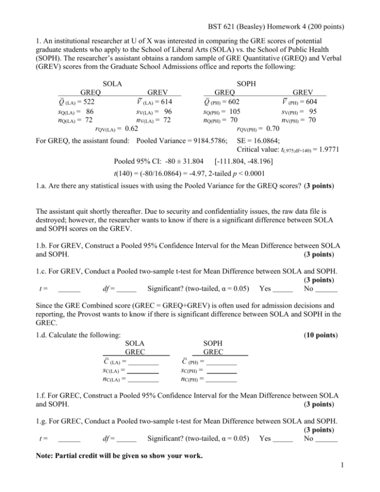
BST 621 (Beasley) Homework 4 (200 points)
1. An institutional researcher at U of X was interested in comparing the GRE scores of potential
graduate students who apply to the School of Liberal Arts (SOLA) vs. the School of Public Health
(SOPH). The researcher’s assistant obtains a random sample of GRE Quantitative (GREQ) and Verbal
(GREV) scores from the Graduate School Admissions office and reports the following:
SOLA
SOPH
GREQ
GREV
(LA) = 614
sQ(LA) = 86
sV(LA) = 96
nQ(LA) = 72
nV(LA) = 72
rQV(LA) = 0.62
Q (LA) = 522
GREQ
Q (PH) = 602
V
sQ(PH) = 105
nQ(PH) = 70
rQV(PH) = 0.70
For GREQ, the assistant found: Pooled Variance = 9184.5786;
Pooled 95% CI: -80 ± 31.804
GREV
(PH) = 604
sV(PH) = 95
nV(PH) = 70
V
SE = 16.0864;
Critical value: t(.975;df=140) = 1.9771
[-111.804, -48.196]
t(140) = (-80/16.0864) = -4.97, 2-tailed p < 0.0001
1.a. Are there any statistical issues with using the Pooled Variance for the GREQ scores? (3 points)
The assistant quit shortly thereafter. Due to security and confidentiality issues, the raw data file is
destroyed; however, the researcher wants to know if there is a significant difference between SOLA
and SOPH scores on the GREV.
1.b. For GREV, Construct a Pooled 95% Confidence Interval for the Mean Difference between SOLA
and SOPH.
(3 points)
1.c. For GREV, Conduct a Pooled two-sample t-test for Mean Difference between SOLA and SOPH.
(3 points)
t=
df =
Significant? (two-tailed, α = 0.05) Yes
No
Since the GRE Combined score (GREC = GREQ+GREV) is often used for admission decisions and
reporting, the Provost wants to know if there is significant difference between SOLA and SOPH in the
GREC.
1.d. Calculate the following:
SOLA
GREC
C (LA) =
sC(LA) =
nC(LA) =
(10 points)
SOPH
GREC
C (PH) =
sC(PH) =
nC(PH) =
1.f. For GREC, Construct a Pooled 95% Confidence Interval for the Mean Difference between SOLA
and SOPH.
(3 points)
1.g. For GREC, Conduct a Pooled two-sample t-test for Mean Difference between SOLA and SOPH.
(3 points)
t=
df =
Significant? (two-tailed, α = 0.05) Yes
No
Note: Partial credit will be given so show your work.
1
BST 621 (Beasley) Homework 4 (200 points)
2. Suppose a test statistic has a Type I error rate of α = 0.05. That is, 5% of the time the test will reject
the null hypothesis when the null hypothesis is actually true. Now suppose the K=3 tests conducted in
the previous analyses were independent.
2.a. What is the probability of at least one failure,
P(r ≥ 1) = _____________.
(3 points)
2.b. Is it reasonable to assume that these tests were independent? Explain.
(3 points)
3. An obesity researcher wanted to investigate the effects of a 12-week diet and exercise program on
obese women. The participants were N=25 females recruited from a local bariatric physician. All
participants had a body mass index (BMI) in excess of 26. The participants BMI and resting metabolic
rate (RMR) were measure before and after the 12-week program. The data for this is in the Microsoft
Excel file (BST621-Assign4-BMI.xls)
SPSS: Use Analyze-Compare Means-Paired Samples T-Test and
choose PRE and POST variables as pairs
Use Analyze-Compare Means One Sample T Test and use the DIFF variables as Test Variables
JMP: Use Analyze-Matched Pairs enter the PRE and POST variables as Y, Paired Response
Use Analyze-Distributions enter the PRE POST and DIFF variables
Under the DIFF Banner select the Test Means Option
SAS: Use PROC MEANS N MISS MEAN STD VAR STDERR T PROBT;VAR PRE POST DIFF;
Use PROC TTEST; PAIRED PRE*POST; RUN; and
3.a. In symbolic notation, what was the null hypothesis for the previous analysis?
(The null hypothesis was the same for both variables.)
3.b. Enter the following Results.
Pre
BMI
Post
(2 points)
(28 points total)
95% CI (Mean Diff)
Lower Bound
Upper Bound
Mean Diff
Mean
SD
t
p-value
SE(MDiff)
n
r
Pre
RMR
Post
df
95% CI (Mean Diff)
Lower Bound
Upper Bound
Mean Diff
Mean
SD
t
p-value
SE(MDiff)
n
r
df
3.c. For both the BMI and RMR, interpret each 95% CI.
(4 points)
3.d. How would missing data affect the interpretation of these results?
(3 points)
3.e. What other limitations does this study have?
(3 points)
2
BST 621 (Beasley) Homework 4 (200 points)
4. Based on these data, conduct a Power analysis for the RMR results. (Daniel, Section 7.9)
Use SAS:
proc power; pairedmeans test=diff
OR
pairedmeans = XXX | YYY
corr = 0.4
pairedstddevs = (S1 S2)
npairs = . (VALUE or .)
power = 0.9 (VALUE or .);run;
proc power;
onesamplemeans test=t
mean = 7
stddev = 3
ntotal = 50 (VALUE or .)
power = . (VALUE or .); run
4.a. What was the “Observed Power” for the RMR results at a two-tailed  = 0.05.?
(3 points)
4.b. Holding these data (Means and SDs) constant, what would a future Total Sample Size (N=number
of pairs) need to be for the RMR results to be statistically significant at a two-tailed  = 0.05.?
(3 points)
4.c. Holding these data (Means and SDs) constant, what would a future Total Sample Size (N=number
of pairs) need to be for the RMR analysis to have 80% Power (1 –  = 0.80) at a two-tailed  = 0.05.?
(3 points)
4.d. Given YOUR DECISION on whether or not to Reject the Null Hypothesis for RMR, what is the
Probability of a Type I Error?
(3 points)
4.e. Given YOUR DECISION on whether or not to Reject the Null Hypothesis for RMR, what is the
Probability of a Type II Error?
(3 points)
5. Write a brief interpretation of these results.
(5 points)
6. Suppose a researcher was interested in doing a research study on the change in Glucose level after
taking metformin among Diabetics. She finds a report from her clinic showing the Mean, Standard
Deviation, sample size (n), and fortunately the correlation (r) for the Blood Glucose Level for n=20
patient Before and After taking metformin :
(14 points)
6.a. Fill in the blanks
Before
BGL
Mean 218
SD
52
After
175
50
95% CI
Lower Bound
Upper Bound
Mean Diff
t
p-value
SE(MDiff)
n
20
20
r
0.65
df
6.b. What was the “Observed Power” for the BGL results at a two-tailed  = 0.05?
(3 points)
6.c. Holding these data (Means and SDs) constant, what would a future Total Sample Size (N=number
of pairs) need to be for the BGL analysis to have 80% Power (1 –  = 0.80) at a two-tailed  = 0.05.?
(3 points)
6.d. Holding these data (Means and SDs) constant, what would a future Total Sample Size (N=number
of pairs) need to be for the BGL analysis to have 80% Power (1 –  = 0.80) at a two-tailed  = 0.01.?
(3 points)
3
BST 621 (Beasley) Homework 4 (200 points)
7. Based on Schwartz et al. (1991), a researcher investigated the effect of cigarette smoking on lung
functioning in patients with idiopathic pulmonary fibrosis. The researcher collected the patient’s
smoking history and measured their percent predicted residual volume (PPRE).
Never
65
100
82
57
84
86
90
107
94
Former
120
60
52
80
103
Directions for 7.b. – 7.d.
Current SPSS: Use Analyze-Compare Means –One Way ANOVA and
105
Select PPRE as the Dependent Variable and Group as Factor
99
Select Options – Descriptive statistics, Homogeneity of Var Test, Welch
103
Select Post-Hoc and Check the Tukey option
104
JMP: Change the X variable to Nominal, then Use Analyze-Fit Y by X
115
Under the Oneway Analysis Banner select the
107
Means/Anova/Pooled t and Means and Std Dev
109
Compare Means – All Pairs, Tukey HSD options
SAS: Use PROC GLM; CLASS group; model PPRE = group / solution;
MEANS group / tukey; RUN;
7.a. State the omnibus null hypotheses for this one-way analysis of variance (ANOVA).
(3 points).
7.b. Complete the ANOVA Source Table with SS, df, MS, and F, and test the null hypothesis in (1) at
the  = .05 level of significance.
(5 points)
Source
SS
df
Between
______
___
MS
F
p-value
_____
____
_____
Within
_______
___
_____
___________________________________________________________________________
Total
________
___
7.c. What is the Model R2? R2 = _______
(2 points)
7.d. Compute Tukey HSD for each pairwise comparison.
Mean Diff
Lower Bound
Never vs Former
Never vs Current
Current vs Former
(9 points).
Upper Bound
7.e. Based on these results explain which groups are significantly different and which group if any has
worse lung functioning.
(4 points).
8. Do you think there is a causal relationship between these variables? Explain.
(3 points).
9.a. What was the “Observed Power” for these results at a two-tailed  = 0.05?
(3 points)
9.b. Holding these data (Means and SDs) constant, what would a future Total Sample Size (N) need to
be for a similar to have 80% Power (1 –  = 0.80) at a two-tailed  = 0.05.?
(3 points)
10. Write a brief interpretation of these results.
(4 points)
4